Visium guided tutorial

Julie Bavais & Denis Puthier

2025-04-15

Working with spatial transcriptomics datasets

The scigenex package offers a certain number of functions dedicated to spatial transcriptomic data analysis. At the moment these functions have been mainly developed to analyse VISIUM technology (10X Genomics).

Searching for gene modules

Pre-process spatial transcriptomics data

Here we will use the stxBrain dataset as example. This dataset is available from SeuratData library and contains mouse brain spatial expression over in several datasets. Two datasets are for the posterior region, two for the anterior. We will use the anterior1 dataset that we will first pre-process using Seurat.

library(Seurat)

## Loading required package: SeuratObject

## Loading required package: sp

## 'SeuratObject' was built under R 4.4.0 but the current version is
## 4.4.1; it is recomended that you reinstall 'SeuratObject' as the ABI
## for R may have changed

## 
## Attaching package: 'SeuratObject'

## The following objects are masked from 'package:base':
## 
##     intersect, t

library(SeuratData)

## ── Installed datasets ──────────────────────────────── SeuratData v0.2.2.9001 ──

## ✔ pbmc3k   3.1.4                        ✔ stxBrain 0.1.2

## ────────────────────────────────────── Key ─────────────────────────────────────

## ✔ Dataset loaded successfully
## ❯ Dataset built with a newer version of Seurat than installed
## ❓ Unknown version of Seurat installed

library(scigenex)

## 

## 

## 

library(ggplot2)
library(patchwork)

suppressWarnings(SeuratData::InstallData("stxBrain"))
brain1 <- LoadData("stxBrain", type = "anterior1")

## Validating object structure

## Updating object slots

## Ensuring keys are in the proper structure
## Ensuring keys are in the proper structure

## Ensuring feature names don't have underscores or pipes

## Updating slots in Spatial

## Updating slots in anterior1

## Validating object structure for Assay5 'Spatial'

## Validating object structure for VisiumV2 'anterior1'

## Object representation is consistent with the most current Seurat version

brain1 <- NormalizeData(brain1, 
                        normalization.method = "LogNormalize",
                        verbose = FALSE)
brain1 <- ScaleData(brain1, verbose = FALSE)
brain1 <- FindVariableFeatures(brain1, verbose = FALSE)
brain1 <- RunPCA(brain1, assay = "Spatial", verbose = FALSE)
brain1 <- FindNeighbors(brain1, reduction = "pca", dims = 1:20, verbose = FALSE)
brain1 <- FindClusters(brain1, verbose = FALSE)
brain1 <- RunUMAP(brain1, reduction = "pca", dims = 1:20, verbose = FALSE)

## Warning: The default method for RunUMAP has changed from calling Python UMAP via reticulate to the R-native UWOT using the cosine metric
## To use Python UMAP via reticulate, set umap.method to 'umap-learn' and metric to 'correlation'
## This message will be shown once per session

DimPlot(brain1, reduction = "umap", label = TRUE)

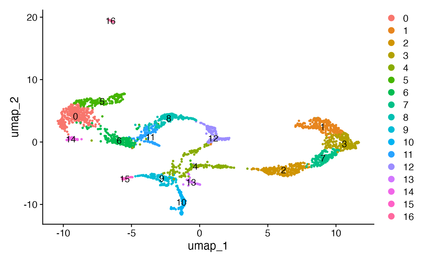
SpatialDimPlot(brain1, label = TRUE, label.size = 3, pt.size.factor = 1.4)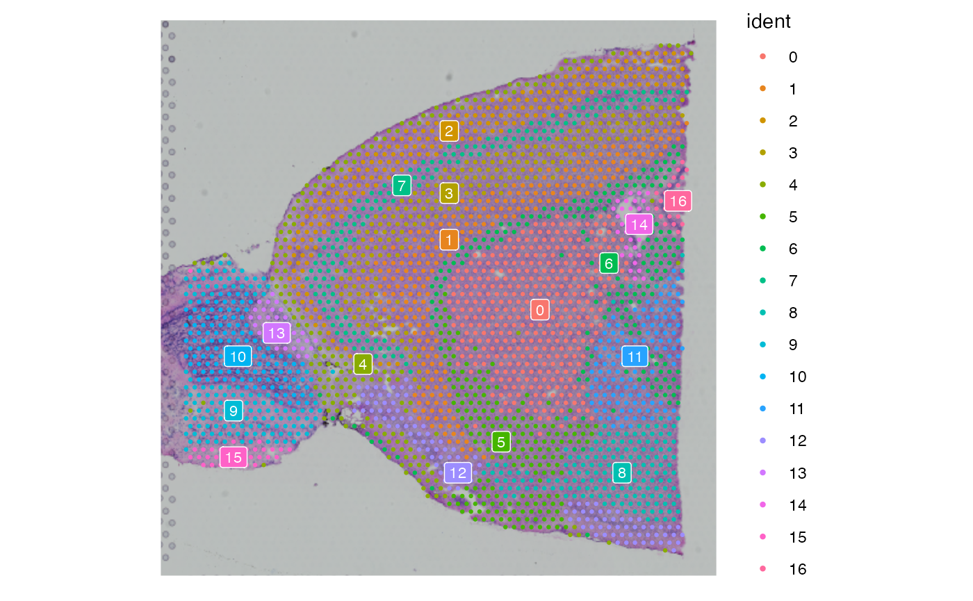

## Scale for fill is already present.
## Adding another scale for fill, which will replace the existing scale.

Calling scigenex

Here we will used the alternative clustering methods proposed by scigenex (“reciprocal_neighborhood”). It is advise to increase slightly k (here k will be set to 80). After call to gene_clustering() we apply filtering on gene modules based on cluster size (min number of genes 7) and standard deviation (gene module sd > 0.1).

set_verbosity(0)
res_brain <- select_genes(data=brain1,
                    k=80,
                    distance_method="pearson",
                    row_sum = 5)

gc_brain <- gene_clustering(res_brain, 
                            method = "reciprocal_neighborhood", 
                            inflation = 2, 
                            threads = 4)

## [1] "MCL path : "

set_verbosity(1)
gcs_brain <- filter_cluster_size(gc_brain, min_cluster_size = 7)

## |-- INFO :  53  clusters with less than 7 were filtered out. 
## |-- INFO :  Number of clusters left 27

df <- cluster_stats(gcs_brain) 
gcss_brain <- gcs_brain[df$sd > 0.1, ]
gcss_brain <- rename_clust(gcss_brain)
length(row_names(gcss_brain))

## [1] 1328

nclust(gcss_brain)

## [1] 27

Interestingly, Scigenex algorithm is able to retrieve nclust(gcss_brain) gene modules. This is most probably reminiscent of cell complexity but also of numerous molecular pathways that are differentially activated across the organ and unanticipated complexity.

Visualizing corresponding heatmap

We then may display the corresponding heatmap using plot_ggheatmap().

set_verbosity(0)
gcss_brain <- top_genes(gcss_brain)
plot_ggheatmap(gcss_brain, 
               use_top_genes = TRUE,
               ident=Idents(brain1)) + ggtitle("All clusters (top genes)") +
               theme(strip.text.y = element_text(size=3))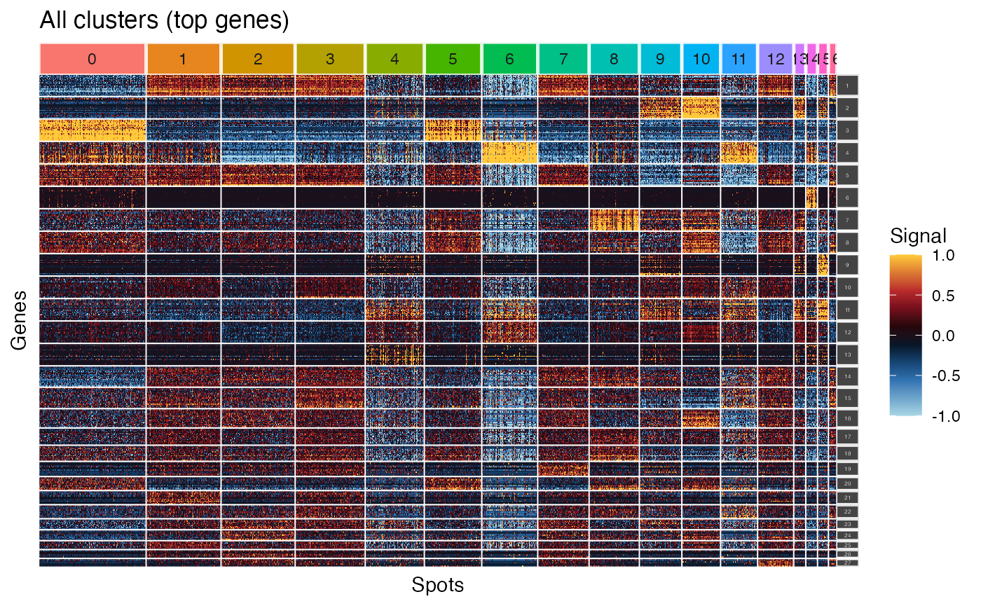

Interactive heatmap

Again, as in the context of scRNA-seq, we may also use the powerful plot_heatmap() fonction which allows interactive exploration of all or specific clusters. Here we look at cluster 1 to 9.

gcss_brain_sub <- subsample_by_ident(gcss_brain, 
                                     nbcell = 30, 
                                     ident =  Seurat::Idents(brain1))

plot_heatmap(gcss_brain_sub[1:9,], 
             use_top_genes = TRUE, 
             cell_clusters = Seurat::Idents(brain1))

# Try selecting a subset of columns/rows
# The 'home' button can be used to reset
# the heatmap

Visualizing topological clusters

The scigenex library implements the plot_spatial() function to display topological information. In addition to the signal, specific regions can be highlighted using a hull that can be created using the display_hull() function. Here will also add a hull around seurat cluster 0 and 2. We will then display signal for “seurat_clusters” metadata.

hull_white <- display_hull(getFlippedTissueCoordinates(brain1),
                           ident = ifelse(Idents(brain1) %in% c(0, 2), 
                                          1, 0),
                           color = "white", 
                           size_x=4, size_y=3, 
                           hull_type = "wall", 
                           size = 0.5, 
                           step_x = 2.6, 
                           step_y=2.4, 
                           delta = 1.5)

plot_spatial(seurat_obj = brain1, 
             metadata = "seurat_clusters", 
             pt_size=2.5, coord_flip = T) + hull_white

We may also want to visualize a specific gene. Here we will look at the pattern of “Hpca” which is part of the cluster 3 detected by Scigenex.

"Hpca" %in% gcss_brain

## [1] TRUE

Hpca_clust <- which_clust( gcss_brain, "Hpca")
Hpca_clust

## Hpca 
##    3

To this aim we will use the plot_spatial() function.

plot_spatial(seurat_obj = brain1, 
             gene_name = "Hpca",  
             pt_size=2.5, coord_flip = T) + hull_white  +
  ggtitle("Hpca expression pattern.")

Note that cluster 3 also contains several genes related to Regulator Of G Protein family. This can be checked with a regular expression using the grep_clust() function:

grep_clust(gcss_brain[Hpca_clust, ], "^Rgs")

## $`3`
## [1] "Rgs9"   "Rgs7bp" "Rgs8"

To visualize the topological distribution of signals in each cluster, we’ll (i) extract the gene_clusters slot from the gcss object, (ii) calculate the module score using Seurat’s AddModuleScore() function and (iii) store the results in the seurat object. Note that, for each gene module, the signal will be scaled from 0 to 1, allowing us to have a common legend for all plots.

brain1 <- AddModuleScore(brain1, features = gcss_brain@gene_clusters)

for(i in 1:nclust(gcss_brain)){ # Normalizing module scores
  tmp <- brain1[[paste0("Cluster", i, sep="")]] 
  max_tmp <- max(tmp)
  min_tmp <- min(tmp)
  brain1[[paste0("Cluster", i, sep="")]]  <- (tmp[,1] - min(tmp))/(max_tmp - min_tmp)
}

The topological profile of cluster 3 (that contains Hpca, a strong hippocampus marker) is the following:

plot_spatial(seurat_obj = brain1, 
             metadata = paste("Cluster", setNames(Hpca_clust, NULL), sep=""), 
             pt_size=2.5, coord_flip = T) + hull_white

We can easily see that the Hpca-containing gene module pattern is very similar to the Hpca pattern. However, the analysis suggests a more complex tissue architecture than expected, as the Hpca signal extends beyond Seurat’s cluster 0.

We will then display the topological signal of all clusters using the plot_spatial_panel() function.

p <- plot_spatial_panel(brain1, 
                        metadata = paste("Cluster", 1:nclust(gcss_brain), 
                                         sep=""), 
                   ncol_layout = 3, 
                   pt_size=0.7, 
                   guide='collect',
                   stroke = 0, size_title = 5, 
                   face_title = 'plain', 
                   barwidth = 0.25, barheight = 1.5, 
                   coord_flip=T) 
print(p + guide_area())

Comparing FindAllMarkers() and Scigenex gene modules

The SciGeneX package propose several functions to evaluate to compare gene sets. They can be handy to compare, for instance, the clusters from two ClusterSet objects (e.g. obtained with different parameters). We may

It may be interesting to compare the clusters obtained using an unsupervised approach (SciGeneX) with those obtained from Seurat::FindAllMarkers(), which searches for genes differentially expressed between cell populations deduced by Seurat::FindClusters().

As shown using the plot_cmp_genesets() function, Seurat::FindAllMarkers() tends to find markers that are not so specific to cell populations. Thus this markers are shared between gene modules. The size of the square is related to the Jaccard index.

seurat_brain_mk <- Seurat::FindAllMarkers(brain1)
seurat_brain_mk<- split(seurat_brain_mk$gene, seurat_brain_mk$cluster)
plot_cmp_genesets(seurat_brain_mk, seurat_brain_mk, layout = "square", transform="-log10" ) + 
  xlab("Seurat::FindAllMarkers()") + 
  ylab("Seurat::FindAllMarkers")

In contrast, gene partitioning in Scigenex is a hard clustering method (elements are not shared between clusters).

plot_cmp_genesets(gcss_brain@gene_clusters, gcss_brain@gene_clusters, layout = "square", transform="-log10") + 
  xlab("Scigenex") + 
  ylab("Scigenex") 

When comparing both (here using hypergeometric) one can see that, although some overlaps exist between gene clusters obtained from both approaches, they are capturing different information that are probably complementary.

plot_cmp_genesets(gcss_brain@gene_clusters, seurat_brain_mk, layout = "raster", stat="hypergeom", transform="-log10" )  +
  ylab("Seurat::FindAllMarkers()") + 
  xlab("Scigenex")