scRNA-seq guided tutorial
Julie Bavais & Denis Puthier
2025-10-15
Source:vignettes/usage.Rmd
usage.RmdGuided tutorial
The easiest way to use scigenex is to perform the following steps using the Seurat R package:
- Load data into a Seurat object
- Perform quality control
- Perform normalization
The resulting object can be used as input to SciGeneX. You can also provide a normalized matrix as input.
The dataset
For this tutorial, we’ll be using a peripheral blood mononuclear cell
(PBMC) scRNA-seq dataset available from the 10x Genomics website. This
dataset contains 2700 individual cells sequenced on the Illumina NextSeq
500 and can be downloaded from
10X Genomics web site or via the SeuratData
library.
Preparing the pbmc3k dataset
In this step, we’ll carry out the classic pre-processing steps of the tutorial. Please refer to this tutorial for more information. If you have already pre-processed your data with Seurat, or if you have a normalized count matrix as input, you can skip this step.
library(ggplot2)
library(patchwork)
library(Seurat, quietly = TRUE)
library(SeuratData)

InstallData("pbmc3k")
data("pbmc3k")
pbmc3k <- UpdateSeuratObject(object = pbmc3k)
We next run the classical steps of the seurat pipeline. For more information, you can check Seurat website here.
# Quality control
pbmc3k[["percent.mt"]] <- PercentageFeatureSet(pbmc3k, pattern = "^MT-")
pbmc3k <- subset(pbmc3k, subset = percent.mt < 5 & nFeature_RNA > 200)

# Normalizing
pbmc3k <- NormalizeData(pbmc3k)

# Identification of highly variable genes
pbmc3k <- FindVariableFeatures(pbmc3k, selection.method = "vst", nfeatures = 2000)

# Scaling data
pbmc3k <- ScaleData(pbmc3k, features = rownames(pbmc3k), verbose = FALSE)

# Perform principal component analysis
pbmc3k <- RunPCA(pbmc3k, features = VariableFeatures(object = pbmc3k), verbose = FALSE)

# Cell clustering
pbmc3k <- FindNeighbors(pbmc3k, dims = 1:10, verbose = FALSE)
pbmc3k <- FindClusters(pbmc3k, resolution = 0.5, verbose = FALSE)

# Dimension reduction
pbmc3k <-suppressWarnings(RunUMAP(pbmc3k, dims = 1:10, verbose = FALSE))
dim_plot_orig <- DimPlot(pbmc3k, reduction = "umap")
dim_plot_orig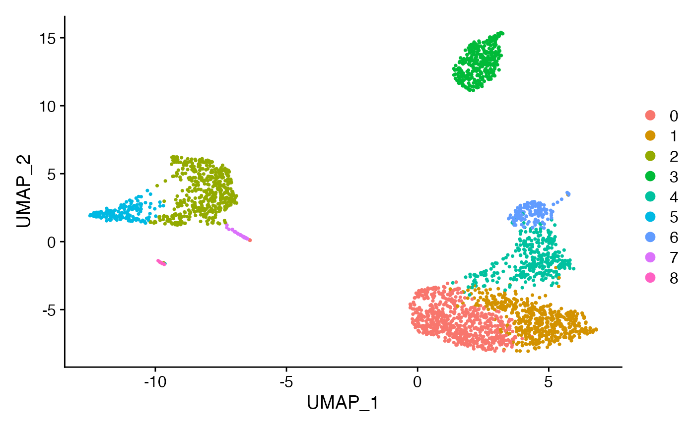
Extracting gene modules using SciGeneX
In this section, we use the previously generated Seurat object as input to run the main SciGeneX commands. This command executes the main algorithm which will:
- identify and extract co-expressed genes
- divide the selected genes into groups
- store the result in a ClusterSet object.
First, we’ll load the SciGeneX library. To limit the verbosity of the SciGeneX functions, we’ll set the verbosity level to zero (which will disable information and debug messages).
library(scigenex)
scigenex::set_verbosity(0)
Then we call successively the select_genes() function
which will select informative genes (i.e co-regulated), then
the gene_clustering() function which will call MCL and
partition the dataset into gene modules.
# Select informative genes
pbmc_scigenex <- select_genes(pbmc3k,
                              k = 50,
                              distance_method = "pearson",
                              layer = "data",
                              row_sum=5)

# Run MCL
pbmc_scigenex <- gene_clustering(pbmc_scigenex,
                                 s = 5,
                                 threads = 2,
                                 inflation = 2)
The object produced is a ClusterSet objet that is a S4
object that is intented to store gene modules.
isS4(pbmc_scigenex)## [1] TRUE
pbmc_scigenex## An object of class ClusterSet
## Name: 89MExU6mw3
## Memory used: 45515040
## Number of cells: 2643
## Number of informative genes: 1793
## Number of gene clusters: 156
## This object contains the following informations:
## - data
## - gene_clusters
## - top_genes
## - gene_clusters_metadata
## - gene_cluster_annotations
## - cells_metadata
## - dbf_output
## - parameters
## * distance_method = pearson
## * k = 50
## * noise_level = 5e-05
## * fdr = 5e-05
## * row_sum = 5
## * no_dknn_filter = FALSE
## * seed = 123
## * keep_nn = FALSE
## * k_graph = 5
## * output_path = /var/folders/zy/wl3dj2_n76zfc8sdvny1q06c0000gn/T//Rtmp332g2g
## * name = 89MExU6mw3
## * inflation = 2
## * algorithm = mclThere are various methods associated with the ClusterSet
objects.
##  [1] "["                        "%in%"
##  [3] "centers"                  "clust_names"
##  [5] "clust_size"               "cluster_set_to_xls"
##  [7] "cluster_stats"            "col_names"
##  [9] "compute_centers"          "dim"
## [11] "enrich_go"                "gene_cluster"
## [13] "grep_clust"               "module_quality_scores"
## [15] "nclust"                   "plot_clust_enrichments"
## [17] "plot_ggheatmap"           "plot_markers_to_clusters"
## [19] "rename_clust"             "reorder_clust"
## [21] "reorder_genes"            "row_names"
## [23] "show"                     "subsample_by_ident"
## [25] "top_by_go"                "top_by_grep"
## [27] "top_by_intersect"         "top_genes"
## [29] "viz_enrich"               "which_clust"
## [31] "write_clust"
The current object contains 1793 informative genes, 2643 samples and 156 gene modules.
nrow(pbmc_scigenex)## [1] 1793
ncol(pbmc_scigenex)## [1] 2643
nclust(pbmc_scigenex)## [1] 156At this stage, several modules need to be filtered, as many of them
may be singletons. Interestingly, the ClusterSet class
implements the indexing operator/function (“[”). The first
argument/dimension of the indexing function corresponds to the cluster
stored in the object. The second dimension corresponds to the cell/spot
names. As an example, we can simply store gene modules whose size
(*i.e. number of genes) is greater than 7 using the following code. The
result is an object containing gene modules 29.
pbmc_scigenex <- pbmc_scigenex[clust_size(pbmc_scigenex) > 7, ]
nclust(pbmc_scigenex)
## [1] 29It may also be important to filter out gene based on dispersion.
Several parameters can be computed for each cluster using the
cluster_stats()function.
plot_cluster_stats(cluster_stats(pbmc_scigenex)) +
 ggplot2::theme(axis.text.y = ggplot2::element_blank(),
                axis.text.x = element_text(angle=45, vjust = 0.5),
panel.grid = element_blank()) 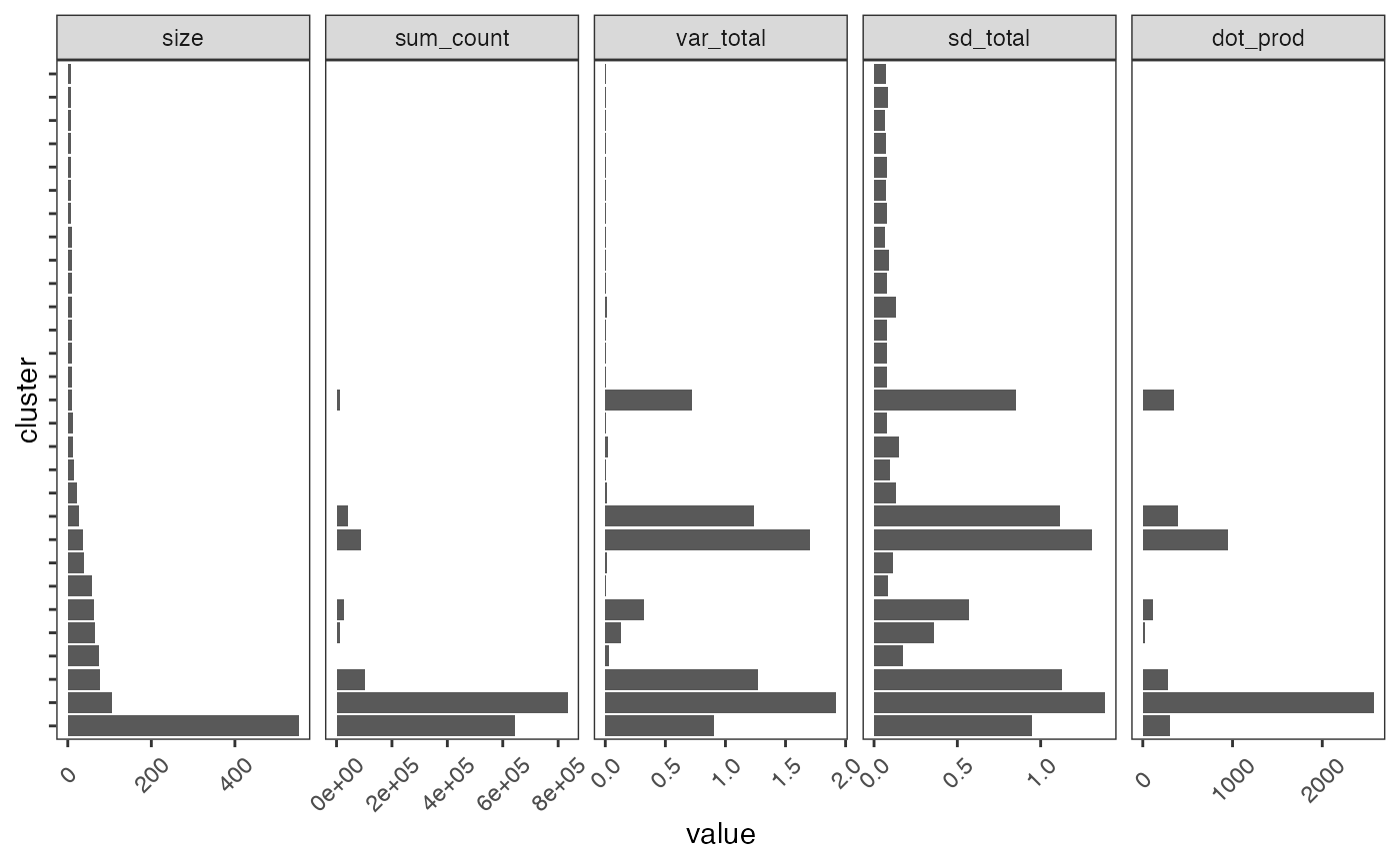
Here we will select gene modules based on standard deviation (> 0.1) and rename the cluster (from 1 to the number of clusters):
pbmc_scigenex <- pbmc_scigenex[cluster_stats(pbmc_scigenex)$sd > 0.1, ]
pbmc_scigenex <- rename_clust(pbmc_scigenex)
nclust(pbmc_scigenex)
## [1] 13Then we check the statistics again.
plot_cluster_stats(cluster_stats(pbmc_scigenex)) +
 ggplot2::theme(axis.text.y = ggplot2::element_blank(),
                axis.text.x = element_text(angle=45, vjust = 0.5),
panel.grid = element_blank()) 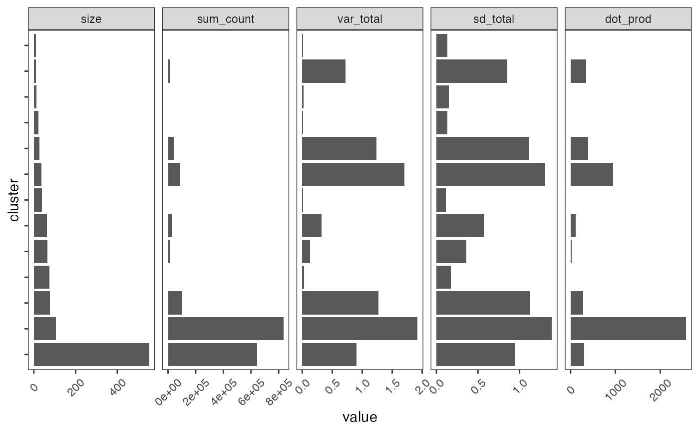
Clusters of genes are stored in the gene_clusters slot.
One can access the gene names from a cluster using the
get_genes() command. By default, all genes are
returned.
# Extract gene names from the 5th gene cluster
genes_module_5 <- get_genes(pbmc_scigenex, cluster = 5)
head(genes_module_5)
## [1] "TMEM40" "GP9" "SDPR" "PF4" "GNG11" "PPBP"One can also access the gene to cluster mapping using
get_genes().
head(gene_cluster(pbmc_scigenex))## CST3 TYROBP AIF1 LST1 LYZ FTL
## 1 1 1 1 1 1
tail(gene_cluster(pbmc_scigenex))## RP4-781K5.2 FNTB C1orf198 SSFA2 ZGLP1 WBP5
## 13 13 13 13 13 13Heatmap visualization
Visualization of specific genetic modules
Visualizing a heatmap containing all cells and modules can be
time-consuming and require significant memory resources. A first
alternative is to examine gene modules individually or a subset of
modules. Gene modules can be visualized using the
plot_heatmap() the plot_ggheatmap() functions.
The former is primarily intended to provide an interactive visualization
based on the iheatmapr library, and allows easy browsing of
results and zooming in on particular regions of the heatmap. This second
solution leads to a diagram that is more easily customized, as it is
based on the ggplot framework. Here, we use
plot_ggheatmap() to view the first 4 clusters. Note that
here, we choose to order the columns/cells on the results of
Seurat::FindClusters.
plot_ggheatmap(pbmc_scigenex[1:4, ],
               use_top_genes = FALSE,
ident=Idents(pbmc3k)) + ggtitle("Cluster 1 to 4") 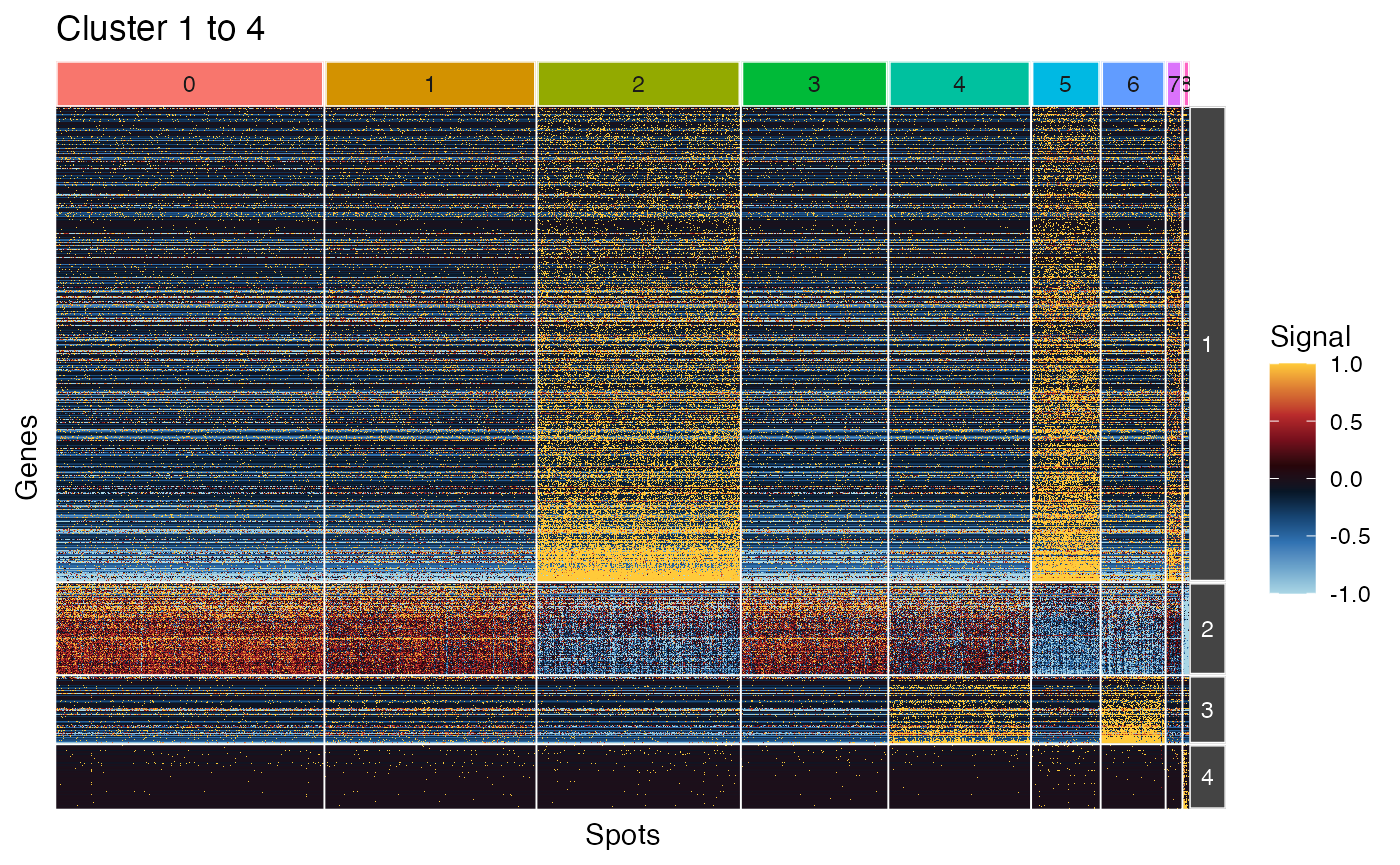
Heatmap of representative genes
However, an alternative is to extract the most representative genes
from each group. This can be achieved using the top_genes()
function. This function stores the identifiers of these representative
genes in the top_genes slot of the ClusterSet
object. The get_genes() function is used to access the
top_genes slot.
pbmc_scigenex <- top_genes(pbmc_scigenex)
genes_cl5_top <- get_genes(pbmc_scigenex, cluster = 5, top = TRUE)
genes_cl5_top
## [1] "GP9" "PF4" "GNG11" "AP001189.4" "SDPR"
## [6] "ITGA2B" "PPBP" "SPARC" "TREML1" "CLU"
## [11] "LY6G6F" "TMEM40" "TUBB1" "SEPT5" "CA2"
## [16] "CMTM5" "HIST1H2AC" "CD9" "MYL9" "GP1BA"Both plot_heatmap() and plot_ggheatmap()
support the use_top_genesargument:
plot_ggheatmap(pbmc_scigenex,
               use_top_genes = TRUE,
               ident=Seurat::Idents(pbmc3k)) + ggtitle("All clusters (top genes)") +
               theme(strip.text.y = element_text(size=4))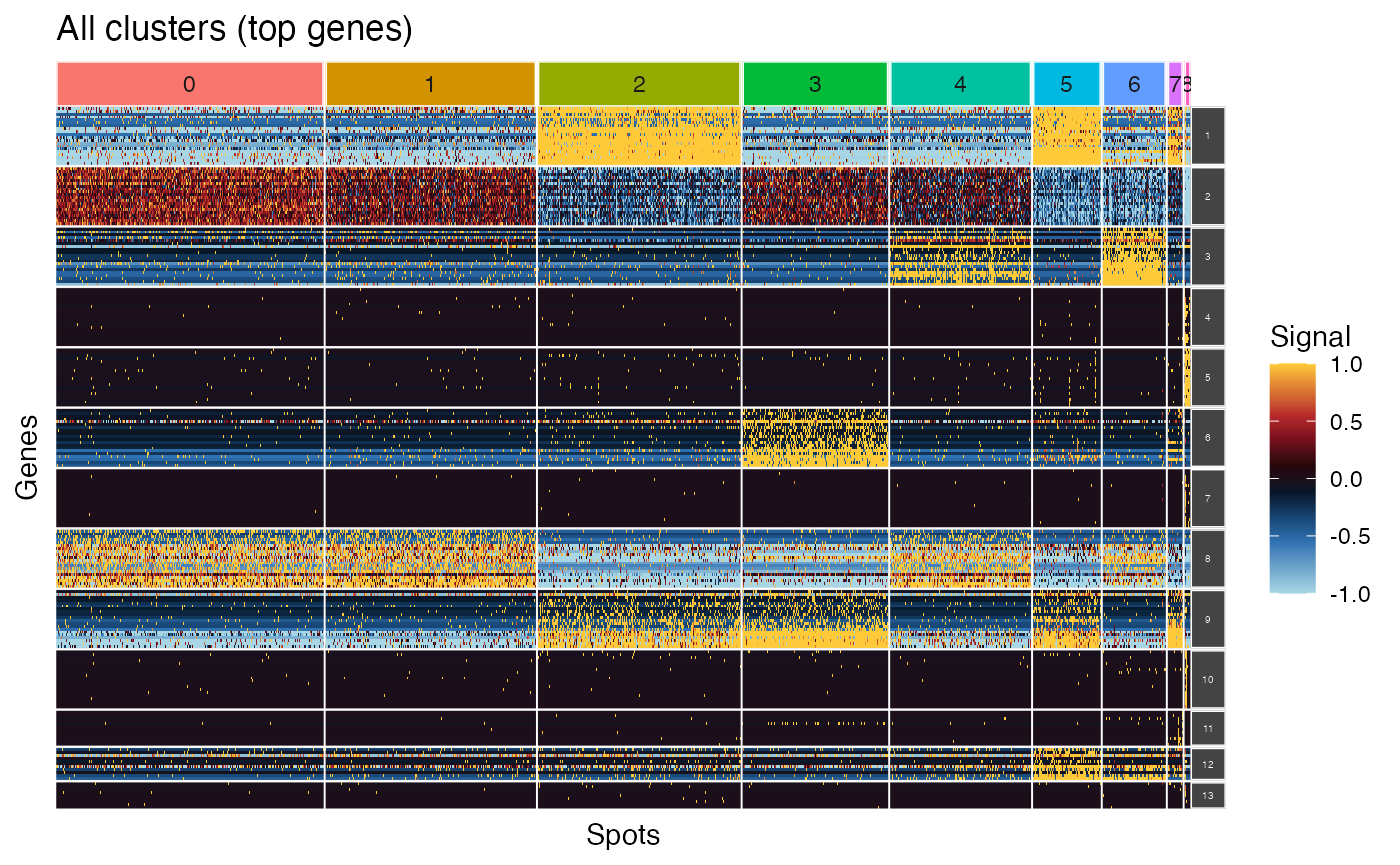
Interactive heatmap
A very interesting feature of SciGeneX is its ability to display gene
expression levels in cells/spots using interactive heatmaps. With this
function, the user can interactively evaluate expression levels in
selected cells or groups, or over the whole dataset. However, it is
generally advisable, when using all clusters, to restrict the analysis
using top_genes=TRUE. Here we will also select a subset of
cells from each cluster.
sub_clust <- subsample_by_ident(pbmc_scigenex,
                                        nbcell=15,
                                        ident=Seurat::Idents(pbmc3k))

plot_heatmap(sub_clust,
            use_top_genes = TRUE,
            cell_clusters =Seurat::Idents(pbmc3k))
Improving cell resolution on UMAP
On can use scigenex selected genes as input for PCA. One can expect some improvement regarding cell population resolution compare to original Seurat pipeline :
# Scaling data using genes from scigenex
pbmc3k <- ScaleData(pbmc3k, features = row_names(pbmc_scigenex), verbose = FALSE)

# Perform principal component analysis
pbmc3k <- RunPCA(pbmc3k, features = VariableFeatures(object = pbmc3k), verbose = FALSE)

# Cell clustering
pbmc3k <- FindNeighbors(pbmc3k, dims = 1:10, verbose = FALSE)
pbmc3k <- FindClusters(pbmc3k, resolution = 0.5, verbose = FALSE)

# Dimension reduction
pbmc3k <-suppressWarnings(RunUMAP(pbmc3k, dims = 1:10, verbose = FALSE))
dim_plot_sci <- DimPlot(pbmc3k, reduction = "umap")

dim_plot_orig + dim_plot_sci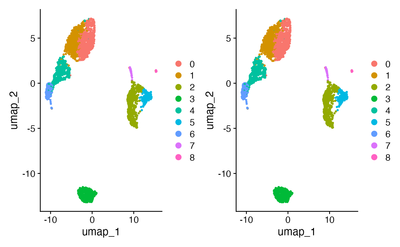
Exporting modules
Gene modules can be exported using the
cluster_set_to_xls(). This function will create a Excel
workbook that will contain the mapping from genes to modules. You may
also use write_clust().
Functional enrichment analysis
Functional enrichment analysis can be performed for each gene module
using the enrich_go() function. Enrichments can be
displayed using the plot_clust_enrichments() function.
# Functional enrichment analysis
pbmc_scigenex <- enrich_go(pbmc_scigenex, specie = "Hsapiens", ontology = "BP")
plot_clust_enrichments(pbmc_scigenex, gradient_palette=colors_for_gradient("Je1"),
                       floor=50,
                       nb_go_term = 2) +
  theme(axis.text.y = element_text(size=4))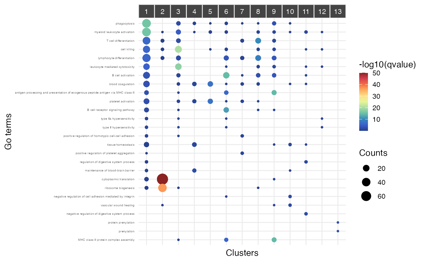
Mapping cell populations markers onto the gene modules
Given a set of markers, the plot_markers_to_clusters()
function can be used to map cell type markers to gene modules. This
function will display jaccard and hypergeometric statistics. Here we
will use the markers from the sctype.app database.
sctype <- "https://zenodo.org/record/8269433/files/sctype.app.tsv"
marker_table <- read.table(sctype, head=TRUE, sep="\t")
marker_table <- marker_table %>%
                filter(Tissue == "Immune system") %>%
                filter(!grepl('Pro-|Pre-|HSC|precursor|Progenitor', Cell.type)) %>%
                separate_rows(Marker_genes, convert = TRUE)

markers <- split(marker_table$Marker_genes,
                 marker_table$Cell.type)
plot_markers_to_clusters(pbmc_scigenex,
                         markers=markers, background = rownames(pbmc3k))
## Warning: The `size` argument of `element_rect()` is deprecated as of ggplot2 3.4.0.
## ℹ Please use the `linewidth` argument instead.
## ℹ The deprecated feature was likely used in the scigenex package.
## Please report the issue to the authors.
## This warning is displayed once every 8 hours.
## Call `lifecycle::last_lifecycle_warnings()` to see where this warning was
## generated.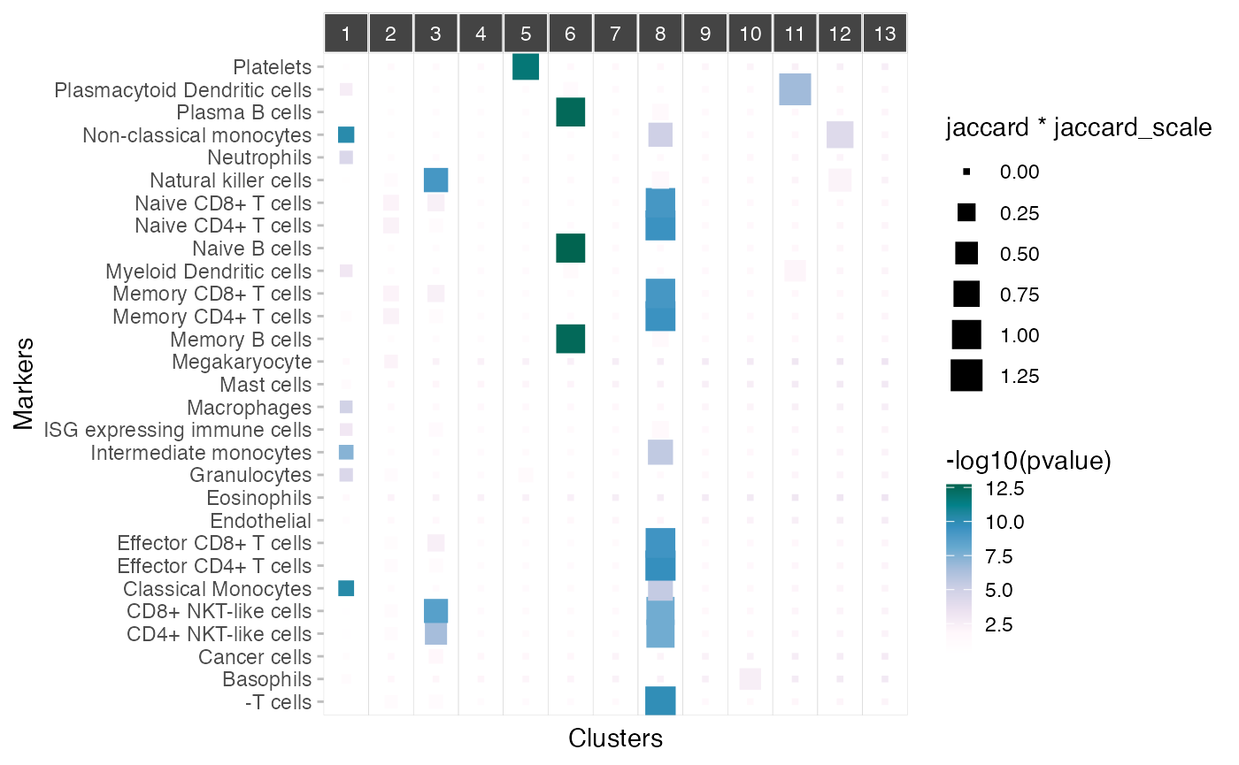
Using scigenex selected genes to improve UMAP
One can restrict PCA computation to the subset of genes selected by
Scigenex. One can expected a significant improvement of segregation of
cell populations. To do so one needs to provide the list of genes
selected by scigenex to the ScaleData() function of Seurat.
A indicated in the RunPCA() help function : “PCA will be run using the
variable features for the Assay. Note that the features must be present
in the scaled data. Any requested features that are not scaled or have 0
variance will be dropped, and the PCA will be run using the remaining
features.”
# Scaling data
feature_2_scale <- row_names(pbmc_scigenex)
pbmc3k_alt <- ScaleData(pbmc3k, features = feature_2_scale, verbose = FALSE)

# Perform principal component analysis
pbmc3k_alt <- RunPCA(pbmc3k_alt, features = VariableFeatures(object = pbmc3k_alt), verbose = FALSE)

# Cell clustering
pbmc3k_alt <- FindNeighbors(pbmc3k_alt, dims = 1:10, verbose = FALSE)
pbmc3k_alt <- FindClusters(pbmc3k_alt, resolution = 0.5, verbose = FALSE)

# Dimension reduction
pbmc3k_alt <-suppressWarnings(RunUMAP(pbmc3k_alt, dims = 1:10, verbose = FALSE))

# Compare alternative projection (pbmc3k_alt) to original (pbmc3k)
DimPlot(pbmc3k, reduction = "umap") + DimPlot(pbmc3k_alt, reduction = "umap") 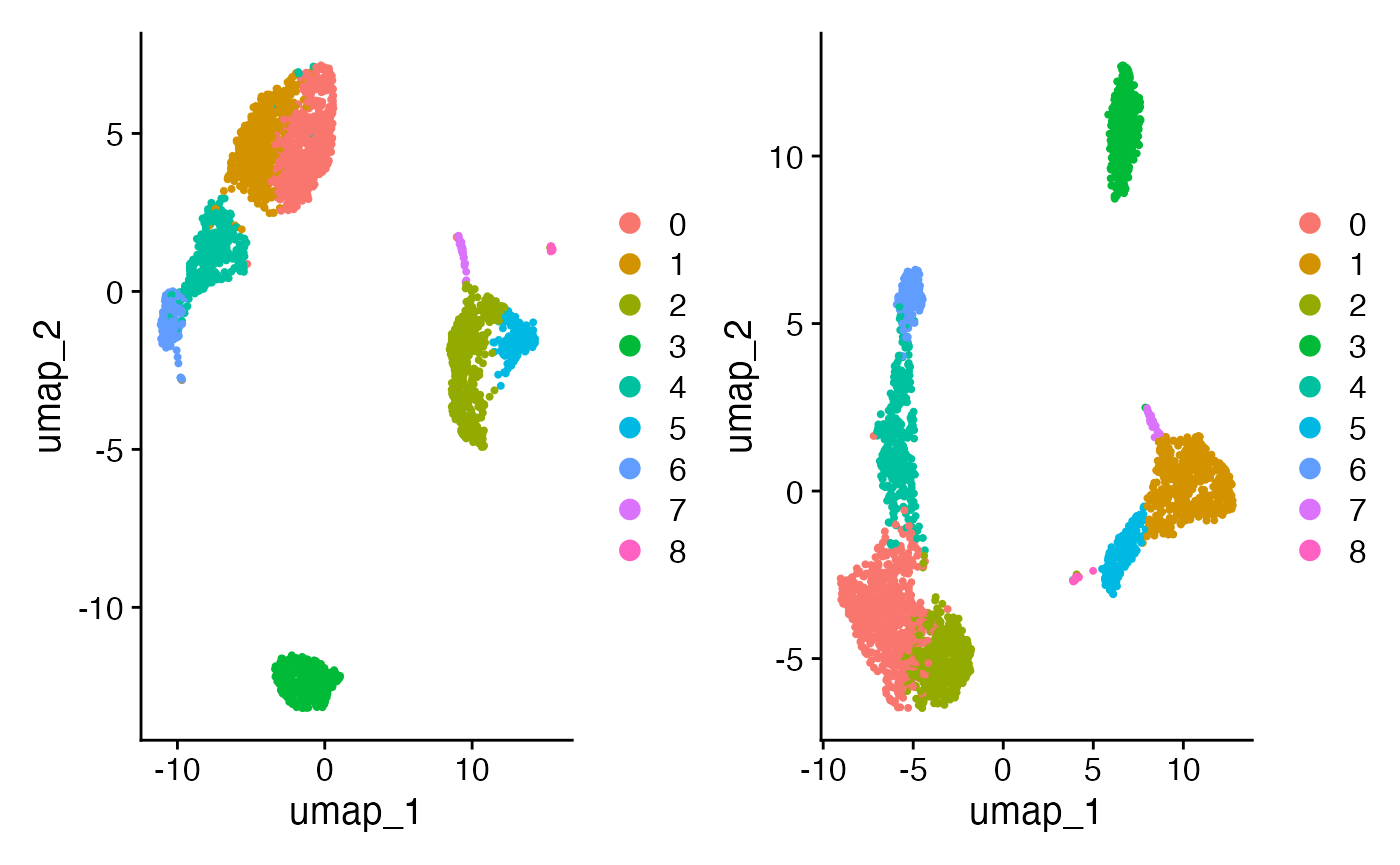
Creating a report
A report can be created using the cluster_set_report()
function. The arguments to this function are the processed clusterSet
and the corresponding processed Seurat object. Ideally, the clusterSet
object should contain functional annotations (see
enrich_go()). Currently, the process of creating a report
can be quite time consuming It can also produce heavy html files which
may take some time to load in the web browser.
# Uncomment to prepare the report.
# gcss_brain <- enrich_go(gcss_brain, species = "Mmusculus", ontology = "BP")
# cluster_set_report(clusterset_object = gcss_brain, seurat_object = brain1)
Session info
## R version 4.4.1 (2024-06-14)
## Platform: x86_64-apple-darwin20
## Running under: macOS Sonoma 14.3.1
##
## Matrix products: default
## BLAS:   /Library/Frameworks/R.framework/Versions/4.4-x86_64/Resources/lib/libRblas.0.dylib
## LAPACK: /Library/Frameworks/R.framework/Versions/4.4-x86_64/Resources/lib/libRlapack.dylib;  LAPACK version 3.12.0
##
## locale:
## [1] en_US.UTF-8/en_US.UTF-8/en_US.UTF-8/C/en_US.UTF-8/en_US.UTF-8
##
## time zone: Europe/Paris
## tzcode source: internal
##
## attached base packages:
## [1] stats     graphics  grDevices utils     datasets  methods   base
##
## other attached packages:
##  [1] tidyr_1.3.1               dplyr_1.1.4
##  [3] scigenex_2.3.0            stxBrain.SeuratData_0.1.2
##  [5] pbmc3k.SeuratData_3.1.4   ifnb.SeuratData_3.1.0
##  [7] SeuratData_0.2.2.9001     Seurat_5.3.0
##  [9] SeuratObject_5.0.2        sp_2.1-4
## [11] patchwork_1.3.2           ggplot2_4.0.0
##
## loaded via a namespace (and not attached):
##   [1] fs_1.6.5                 matrixStats_1.4.1        spatstat.sparse_3.1-0
##   [4] enrichplot_1.24.4        httr_1.4.7               RColorBrewer_1.1-3
##   [7] docopt_0.7.1             tools_4.4.1              sctransform_0.4.1
##  [10] R6_2.6.1                 DT_0.33                  lazyeval_0.2.2
##  [13] uwot_0.2.2               withr_3.0.2              clValid_0.7
##  [16] prettyunits_1.2.0        gridExtra_2.3            progressr_0.14.0
##  [19] cli_3.6.4                Biobase_2.64.0           textshaping_0.4.0
##  [22] spatstat.explore_3.3-2   fastDummies_1.7.4        scatterpie_0.2.4
##  [25] slam_0.1-53              labeling_0.4.3           sass_0.4.9
##  [28] S7_0.2.0                 spatstat.data_3.1-2      ggridges_0.5.6
##  [31] pbapply_1.7-2            pkgdown_2.1.1            systemfonts_1.1.0
##  [34] yulab.utils_0.1.7        gemini.R_0.13.1          gson_0.1.0
##  [37] DOSE_3.30.5              R.utils_2.12.3           parallelly_1.38.0
##  [40] WriteXLS_6.7.0           rstudioapi_0.16.0        RSQLite_2.3.7
##  [43] iheatmapr_0.7.1          gridGraphics_0.5-1       generics_0.1.3
##  [46] ica_1.0-3                spatstat.random_3.3-2    GO.db_3.19.1
##  [49] Matrix_1.7-0             S4Vectors_0.42.1         abind_1.4-8
##  [52] R.methodsS3_1.8.2        lifecycle_1.0.4          yaml_2.3.10
##  [55] qvalue_2.36.0            BiocFileCache_2.12.0     Rtsne_0.17
##  [58] grid_4.4.1               blob_1.2.4               promises_1.3.2
##  [61] crayon_1.5.3             miniUI_0.1.1.1           lattice_0.22-6
##  [64] cowplot_1.1.3            KEGGREST_1.44.1          pillar_1.10.1
##  [67] knitr_1.49               fgsea_1.30.0             future.apply_1.11.2
##  [70] codetools_0.2-20         fastmatch_1.1-4          glue_1.8.0
##  [73] ggfun_0.1.6              spatstat.univar_3.0-1    data.table_1.17.0
##  [76] treeio_1.28.0            vctrs_0.6.5              png_0.1-8
##  [79] spam_2.11-0              testthat_3.2.1.1         org.Mm.eg.db_3.19.1
##  [82] gtable_0.3.6             amap_0.8-19.1            cachem_1.1.0
##  [85] xfun_0.53                mime_0.12                tidygraph_1.3.1
##  [88] qlcMatrix_0.9.8          survival_3.7-0           pheatmap_1.0.12
##  [91] fitdistrplus_1.2-1       ROCR_1.0-11              nlme_3.1-166
##  [94] ggtree_3.12.0            bit64_4.6.0-1            progress_1.2.3
##  [97] filelock_1.0.3           RcppAnnoy_0.0.22         GenomeInfoDb_1.40.1
## [100] bslib_0.9.0              irlba_2.3.5.1            KernSmooth_2.23-24
## [103] colorspace_2.1-1         BiocGenerics_0.50.0      DBI_1.2.3
## [106] tidyselect_1.2.1         bit_4.5.0.1              compiler_4.4.1
## [109] curl_5.2.3               httr2_1.0.5              SparseM_1.84-2
## [112] xml2_1.3.6               desc_1.4.3               plotly_4.10.4
## [115] shadowtext_0.1.4         bookdown_0.41            scales_1.4.0
## [118] lmtest_0.9-40            rappdirs_0.3.3           stringr_1.5.1
## [121] digest_0.6.37            goftest_1.2-3            spatstat.utils_3.1-0
## [124] sparsesvd_0.2-2          rmarkdown_2.29           XVector_0.44.0
## [127] base64enc_0.1-3          htmltools_0.5.8.1        pkgconfig_2.0.3
## [130] MatrixGenerics_1.16.0    sparseMatrixStats_1.16.0 dbplyr_2.5.0
## [133] fastmap_1.2.0            rlang_1.1.6              htmlwidgets_1.6.4
## [136] UCSC.utils_1.0.0         shiny_1.10.0             ggh4x_0.3.1.9000
## [139] farver_2.1.2             jquerylib_0.1.4          zoo_1.8-12
## [142] jsonlite_1.9.0           BiocParallel_1.38.0      GOSemSim_2.30.2
## [145] R.oo_1.26.0              magrittr_2.0.4           ggplotify_0.1.2
## [148] GenomeInfoDbData_1.2.12  dotCall64_1.2            Rcpp_1.0.14
## [151] ape_5.8-1                viridis_0.6.5            reticulate_1.39.0
## [154] stringi_1.8.4            ggstar_1.0.4             ggraph_2.2.1
## [157] brio_1.1.5               zlibbioc_1.50.0          MASS_7.3-61
## [160] plyr_1.8.9               org.Hs.eg.db_3.19.1      ggstats_0.9.0
## [163] parallel_4.4.1           listenv_0.9.1            ggrepel_0.9.6
## [166] deldir_2.0-4             Biostrings_2.72.1        graphlayouts_1.2.0
## [169] splines_4.4.1            pander_0.6.6             tensor_1.5
## [172] hms_1.1.3                fastcluster_1.2.6        igraph_2.1.4
## [175] spatstat.geom_3.3-3      RcppHNSW_0.6.0           reshape2_1.4.4
## [178] biomaRt_2.60.1           stats4_4.4.1             evaluate_1.0.3
## [181] BiocManager_1.30.25      tweenr_2.0.3             httpuv_1.6.15
## [184] RANN_2.6.2               purrr_1.1.0              polyclip_1.10-7
## [187] future_1.34.0            scattermore_1.2          ggforce_0.4.2
## [190] xtable_1.8-4             tidytree_0.4.6           RSpectra_0.16-2
## [193] later_1.4.1              viridisLite_0.4.2        class_7.3-22
## [196] ragg_1.3.3               tibble_3.2.1             clusterProfiler_4.12.6
## [199] aplot_0.2.3              memoise_2.0.1            AnnotationDbi_1.66.0
## [202] IRanges_2.38.1           cluster_2.1.6            globals_0.16.3
## [205] xaringanExtra_0.8.0