Guided tutorial

Overview

The STarlight package is an R package designed for the exploratory analysis of cell or molecule coordinates obtained from Spatial omics experiments (e.g. Merscope, Xenium or CosMx). By employing a grid-based approach, STarlight enables to explore the datasets at multiple scales and resolution and to discover spatial patterns and relationships. STarlight also implements various function to perfors multi-sample comparisons and assess the dynamics over biological conditions.

Loading libraries

library(magrittr)
library(Seurat)
library(STarlight)
STarlight::set_verb_level(0)
library(patchwork)
library(ggplot2)
library(dplyr)

Retrieving the dataset

We are going to use a subset (64 genes) of a 10x Genomics dataset taken from the Xenium Explorer Demo. The region corresponds to a fresh frozen mouse brain coronal section. The original dataset can be downloaded here.

## Create a temporary folder
tmpdir <- tempdir()
dir.create(tmpdir, showWarnings = FALSE)
remote_file <- "Xenium_Mouse_Brain_Coronal_tiny.csv.gz"
## Download and unzip the file
url_data <- paste0("https://zenodo.org/records/11371819/files/",
                   remote_file)
dest_file <- file.path(tmpdir, remote_file)
download.file(url_data, destfile = dest_file)

Loading the data

The load_spatial() function is the entry point of the STarlight package. It allows you to load molecule coordinates and create a 2D binned grid (default size of 25µm) that will be stored in an S4 object of class STGrid. Since we are working with a csv flat file containing x/y molecular coordinates and gene names we do not need to specify the argument method. If you have access to the full Xenium directory, you can use the arguments method="xenium" and path="path/to/directory" to load the data.

st_obj <- load_spatial(path = dest_file, 
             method = "coordinates", 
             sep=",", 
             mapping = c(feature="feature_name", 
                         x="x_location", 
                         y="y_location"), 
                         bin_size = 25, 
            control = "(NegControlProbe_)|(BLANK_)", verbose = FALSE)

Side note

Using the argument control in the load_spatial function allows users to identify blank/control probes in their data. The probes can be removed using the command below:

st_obj <- rm_controls(st_obj)

Manipulating the STGrid object

The Spatial Transcriptomic Grid class (STGrid) is a structured framework for managing and analyzing data. It facilitates the exploration and interpretation of spatial gene expression patterns within tissue sections.

STarlight::set_verb_level(1)
st_obj
#> |-- INFO :  An object of class STGrid 
#> |-- INFO :  Number of counts:  2151300 
#> |-- INFO :  Number of features:  61 
#> |-- INFO :  Bin size:  25 
#> |-- INFO :  Number of bins (x axis):  218 
#> |-- INFO :  Number of bins (y axis):  141 
#> |-- INFO :  x_min:  7.1552773 
#> |-- INFO :  x_max:  5447.244 
#> |-- INFO :  y_min:  12.103435 
#> |-- INFO :  y_max:  3534.868 
#> |-- INFO :  >>> Please, use show_st_methods() to show availables methods <<<

Here are the slots contained in the object:

slotNames(st_obj)
#>  [1] "coord"             "bin_mat"           "y_max"            
#>  [4] "y_min"             "x_min"             "x_max"            
#>  [7] "path"              "method"            "meta"             
#> [10] "bin_size"          "bin_x"             "bin_y"            
#> [13] "ripley_k_function" "control"

Multiple methods are supported by the STGrid object:

STarlight::show_st_methods()
#>  [1] "["                    "[["                   "[[<-"                
#>  [4] "$"                    "$<-"                  "as_matrix"           
#>  [7] "bin_mat"              "bin_size"             "bin_x"               
#> [10] "bin_y"                "cc_neighborhood"      "check_features_exist"
#> [13] "col_names"            "compute_k_ripley"     "compute_module_score"
#> [16] "connected_components" "coord"                "create_hull"         
#> [19] "dim"                  "feat_names"           "feature_contrast"       
#> [22] "get_coord"            "hc_tree"              "meta_names"          
#> [25] "meta"                 "multi_feat_contrast"  "nb_feat"             
#> [28] "nb_items"             "nbin_x"               "nbin_y"              
#> [31] "order_feat_by_ripley" "plot_rip_k"           "re_bin"              
#> [34] "ripley_k_function"    "rm_controls"          "row_names"           
#> [37] "show"                 "spatial_image"        "spatial_plot"        
#> [40] "summary"              "tab"                  "table_st"            
#> [43] "write_coord"

Subsetting

We’ve made it easy for users to subset data in their STGrid object using the “[” operator. This is designed to facilitate the extraction of specific genes or regions for a more focused analysis.

Subsetting using bin_x / bin_y

We can explore the binning information stored within the STGrid object using bin_x() and bin_y().

This command retrieves the first few entries of the bin_x vector (bins along the x-axis).

head(bin_x(st_obj))

Similarly, this command retrieves the first few entries of the bin_y vector (bins along the y-axis).

head(bin_y(st_obj))

We can leverage the subsetting function to extract data corresponding to specific bins along the x-axis (i.e. bins from the 50th to the 100th entry of the bin_x vector). The following command extracts a subset of the data and saves it to a new STGrid object.

subset <- st_obj[bin_x(st_obj)[50:100], ]

Subsetting using genes

We can also extract data associated to specific genes. Here we extract data corresponding to the genes Chat and Cbln4:

st_obj[c("Chat", "Cbln4"), ]

Subsetting using numeric indices

We can retrieve data based on the position of genes within the feat_names() vector of the STGrid object. Let’s extract data for the first 10 genes according to their position in the feat_names() vector:

st_obj[feat_names(st_obj)[1:10], ]

Users can also explore data for the 10th to 12th genes using numeric indices. We first start by determining the total number of genes in our STGrid object:

nb_feat(st_obj)

We then retrieve data for genes positioned 10 through 12 in the feat_names() vector.

st_obj[10:12, ]

Visualization functions

The spatial_image() function

The spatial_image() function allows users to visualize the spatial density of molecules across tissue sections. Users can do the following if they want to visualize a single gene. The grid=TRUE argument overlays a bin of a specified size, which eases the selection of particular regions.


 p <- spatial_image(
  st_obj,
  feat = "Ano1",
  grid = 20,
  logb = 10,
  scale = TRUE,
  saturation = 0.9
)

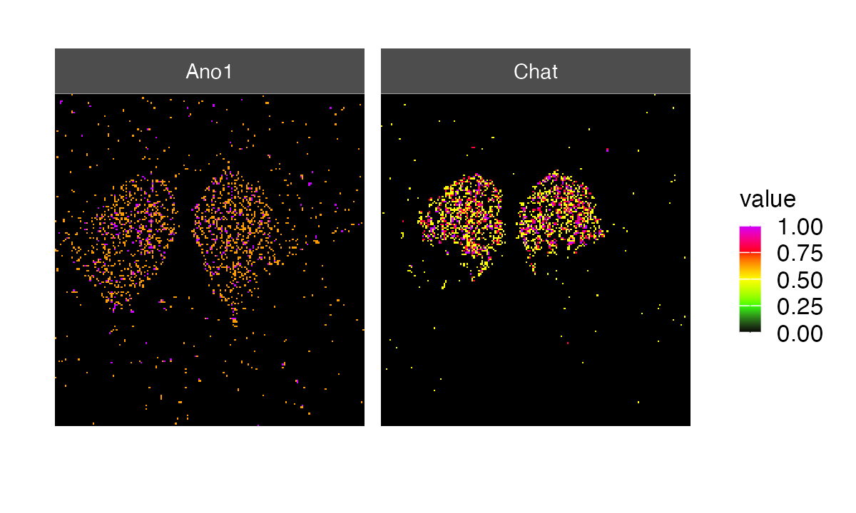
Users can choose to zoom into specific regions. For example, we can zoom into the region with a high Ano1 molecule density (upper right corner of the image above). We use rebin() to increase the binning resolution of the selected region.

x_bins <-  bin_x(st_obj)[181:nbin_x(st_obj)]
y_bins <-  bin_y(st_obj)[101:nbin_y(st_obj)]
st_obj_r1 <- st_obj[x_bins, y_bins]
spatial_image(
  re_bin(st_obj_r1[c("Ano1", "Chat"),], bin_size = 5, verbose = FALSE),
  feat = c("Ano1", "Chat"),
  logb = 10,
  scale = TRUE,
  saturation = 0.9
)

The spatial_plot() function

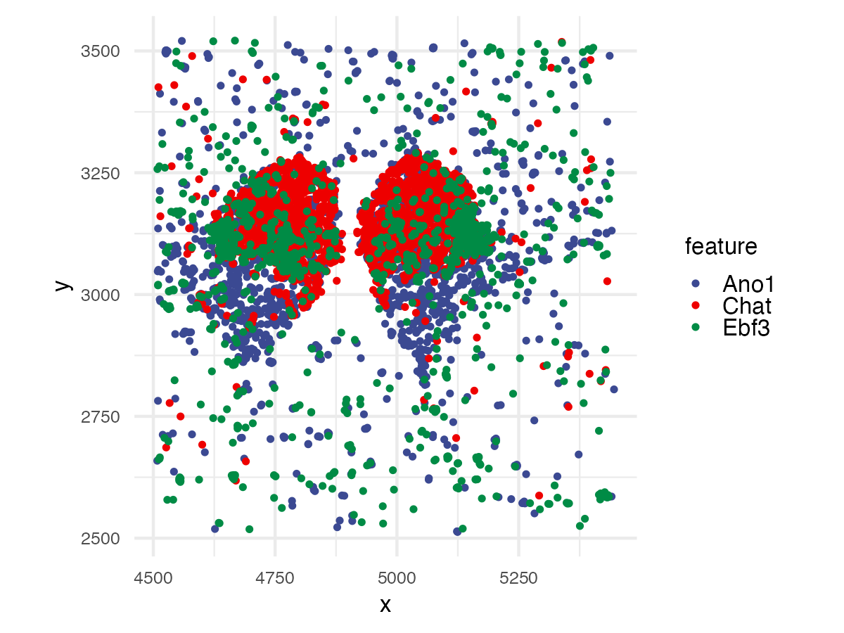
The spatial_plot() function can be used to create scatter plots of molecular x/y coordinates. We can choose to highlight other molecules potentially located in the vicinity of Ano1.

spatial_plot(
  st_obj[x_bins, y_bins],
  feat_list = c("Ano1",
                "Chat",
                "Ebf3"),
  colors = ggsci::pal_aaas()(3),
  size = 0.6
)

The feature_contrast() function

This function can be used to compare the log2 ratio between two genes across x/y bins. Several genes pairs can be provided.


feature_contrast(
  st_obj,
  feat_list_1 = c("Nwd2",
                  "Kctd8",
                  "Chat"),
  feat_list_2 = c("Igf1",
                  "Ebf3", 
                  "Hat1"),
  centered = TRUE, 
  trim_ratio = 0.025)

The multi_feat_contrast() function

This function performs a contrast analysis between multiple features (genes) by binarizing gene expression based on a user-defined threshold across x/y bins. An STGrid object is used as input. For each bin, a binary vector is computed and encoded as a color (e.g 000, none of 3 genes are above the threshold; 100, gene 1 is the only one above the threshold; 110, gene 1 and 2 are both above the threshold…). The number of colors required increases rapidly (2^(length(feat_list))) as the number of genes increases. It is advised not to go beyond 4 features/genes.


multi_feat_contrast(
  st_obj,
  feat_list = c("Ebf3",
                "Kctd8",
                "Chat",
                "Ano1"), 
  threshold = 2)

Neighborhood exploration

Indentifying connected components

Cell populations expressing a specific marker may be found more or less clustered in the tissue. The bins containing the corresponding molecules may appear as connected components that can be captured using the connected_components() function. The connected components are stored in the meta slot of the STGrid object and named with original feature name and a “_cpt” suffix. Here we will search for connected components displaying at least 1 count for Nwd2 filtering out those with surface lower than 9 bins. We will also add a hull around the connected components.

st_obj <- connected_components(st_obj, feat_list = "Nwd2", 
                               threshold = 1, min_size = 9)
nb_cc <- length(unique(st_obj$Nwd2_cpt))
p1 <- spatial_image(st_obj, features = "Nwd2_cpt", 
                    as_factor = TRUE, 
                    colors = c("black", rainbow(nb_cc - 1))) 
p2 <- p1 + create_hull(st_obj, feat = "Nwd2_cpt", color="grey") 
p1 + p2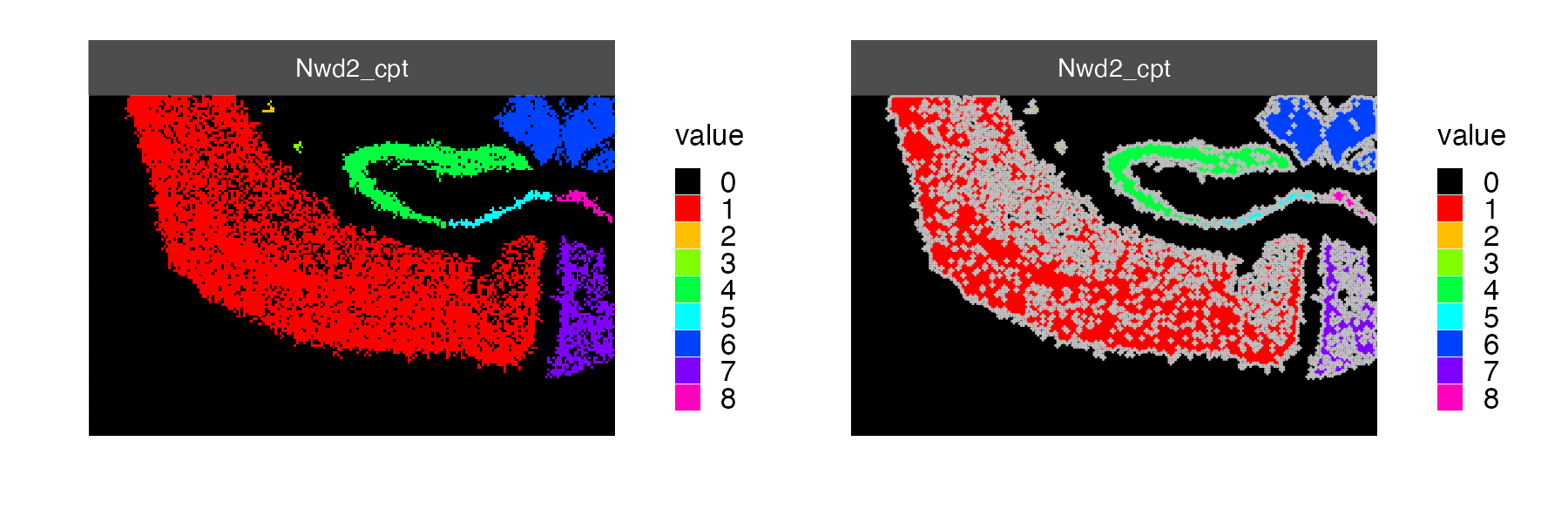

We can next extend the connected component with neighboring bins with the objective to more clearly highlight the component of interest.

st_obj <- cc_neighborhood(st_obj, feat = "Nwd2_cpt")
head(meta(st_obj), 3)
p1 + create_hull(st_obj, feat = "Nwd2_cpt_ngb")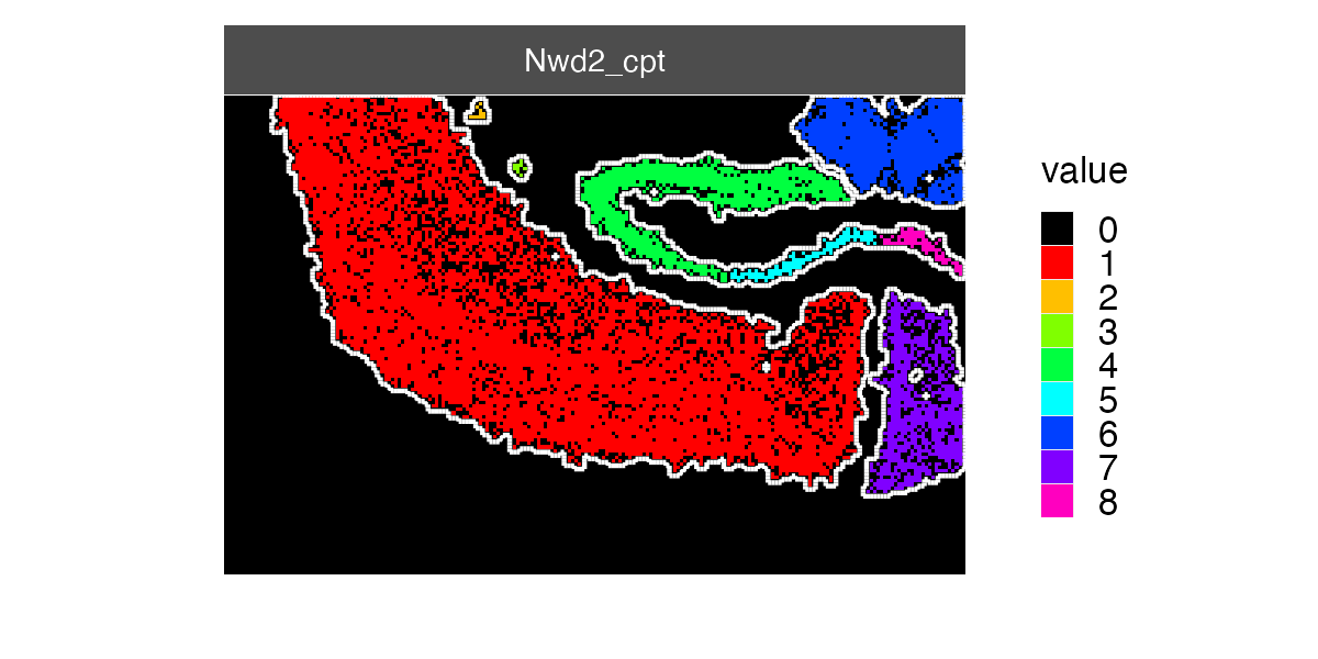

And use this hull as a footprint of Nwd2 gene expression when analysing Cpne4.

spatial_image(st_obj, "Cpne4") + create_hull(st_obj, 
                                             feat = "Nwd2_cpt_ngb", 
                                             linewidth = .3, color="white")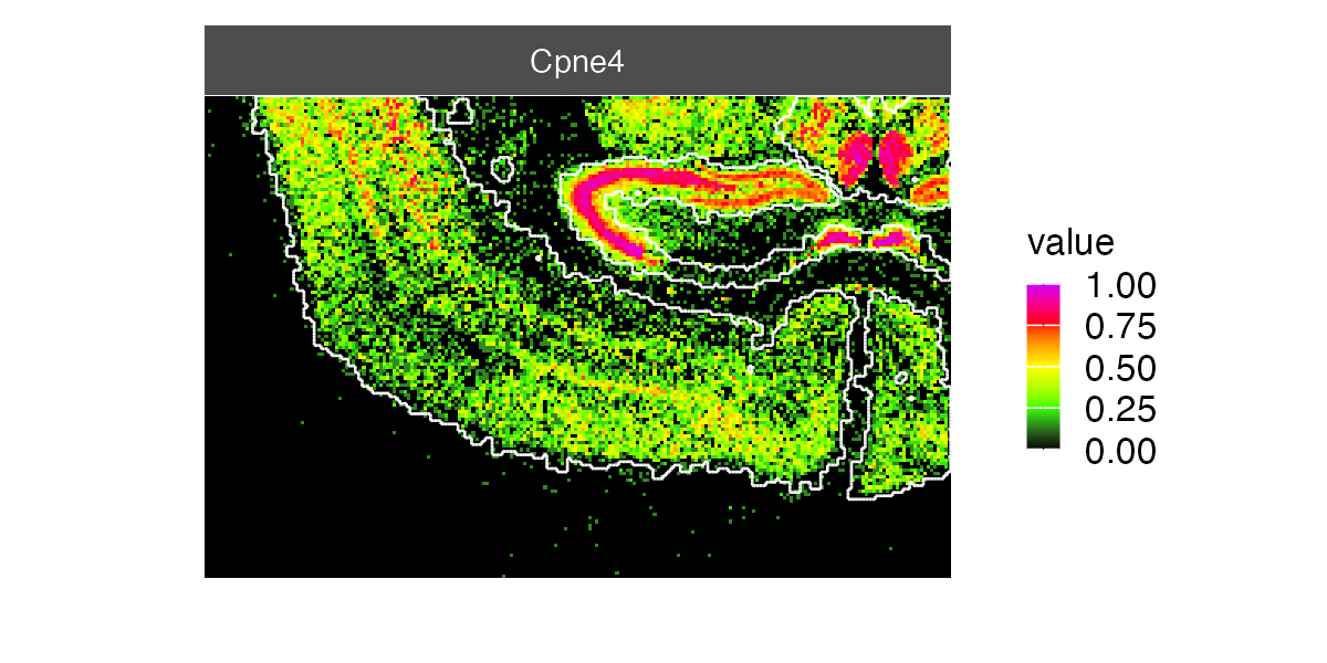

Identifying co-localizing genes

The hc_tree() function can used to organize genes into subclusters (modules), revealing which genes tend to colocalize and follow a similar spatial distribution across the tissue.

hc_st <- hc_tree(
  st_obj,
  method = "ward.D",
  layout = "circular",
  dist_method = "pearson",
  class_nb = 20, 
  lab_fontsize = 2.5,
  offset = 9
) 

hc_st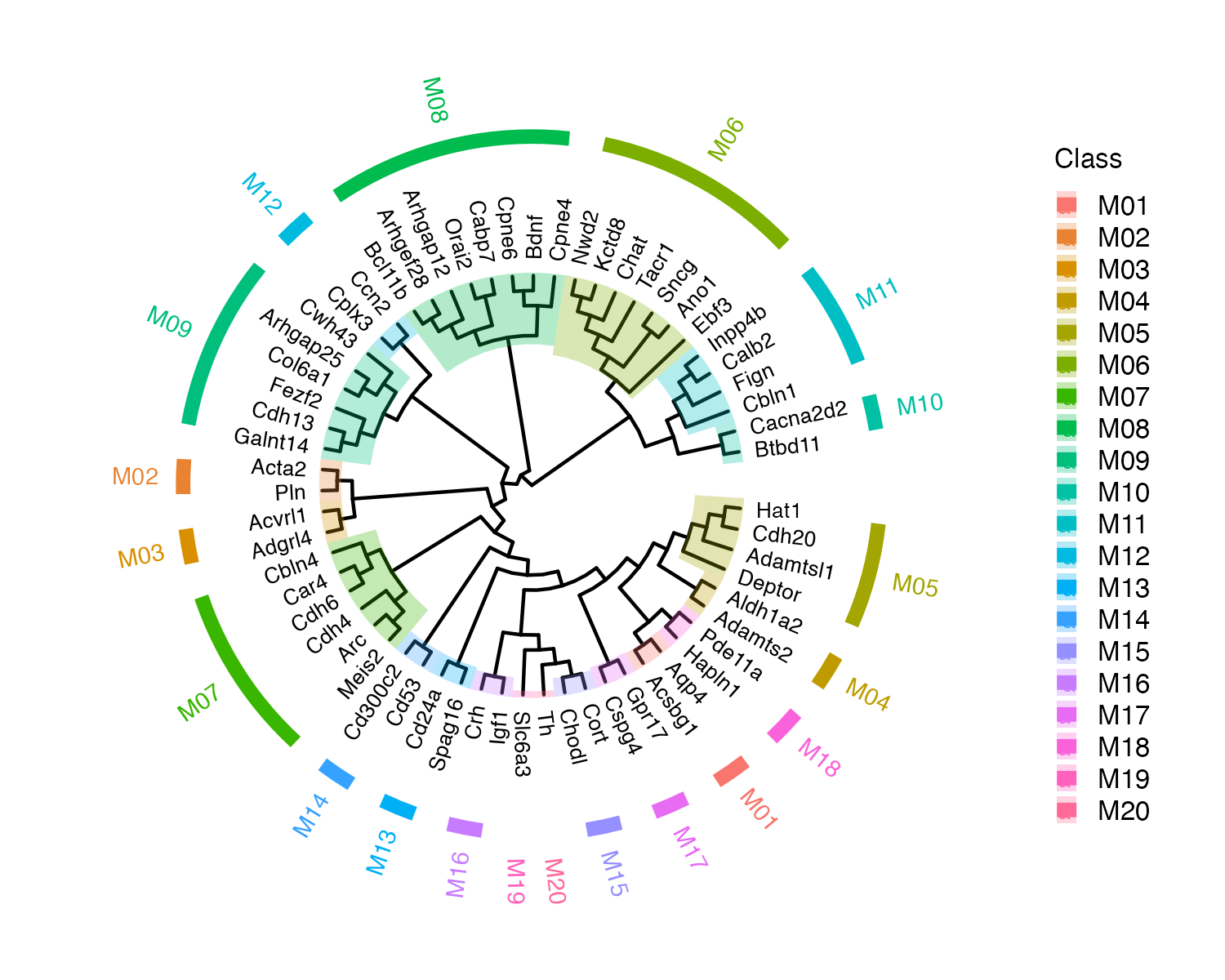

# The first 3 modules
hc_st$tree_classes[1:3]
#> $MOD01
#> [1] "Acsbg1" "Aqp4"  
#> 
#> $MOD02
#> [1] "Acta2" "Pln"  
#> 
#> $MOD03
#> [1] "Acvrl1" "Adgrl4"

Compute average module score.

st_obj <- compute_module_score(st_obj, modules = hc_st$tree_classes)
#> |-- INFO :  Computing module score... 
#> |-- INFO :  Iterating over modules... 
#> |-- INFO :  Returning object...
meta_names(st_obj)
#>  [1] "count_sum"    "Nwd2_cpt"     "Nwd2_cpt_ngb" "MOD01"        "MOD02"       
#>  [6] "MOD03"        "MOD04"        "MOD05"        "MOD06"        "MOD07"       
#> [11] "MOD08"        "MOD09"        "MOD10"        "MOD11"        "MOD12"       
#> [16] "MOD13"        "MOD14"        "MOD15"        "MOD16"        "MOD17"       
#> [21] "MOD18"        "MOD19"        "MOD20"

We can map modules using the spatial_image() function.

spatial_image(st_obj, features = meta_names(st_obj)[-c(1:3)], ncol = 4)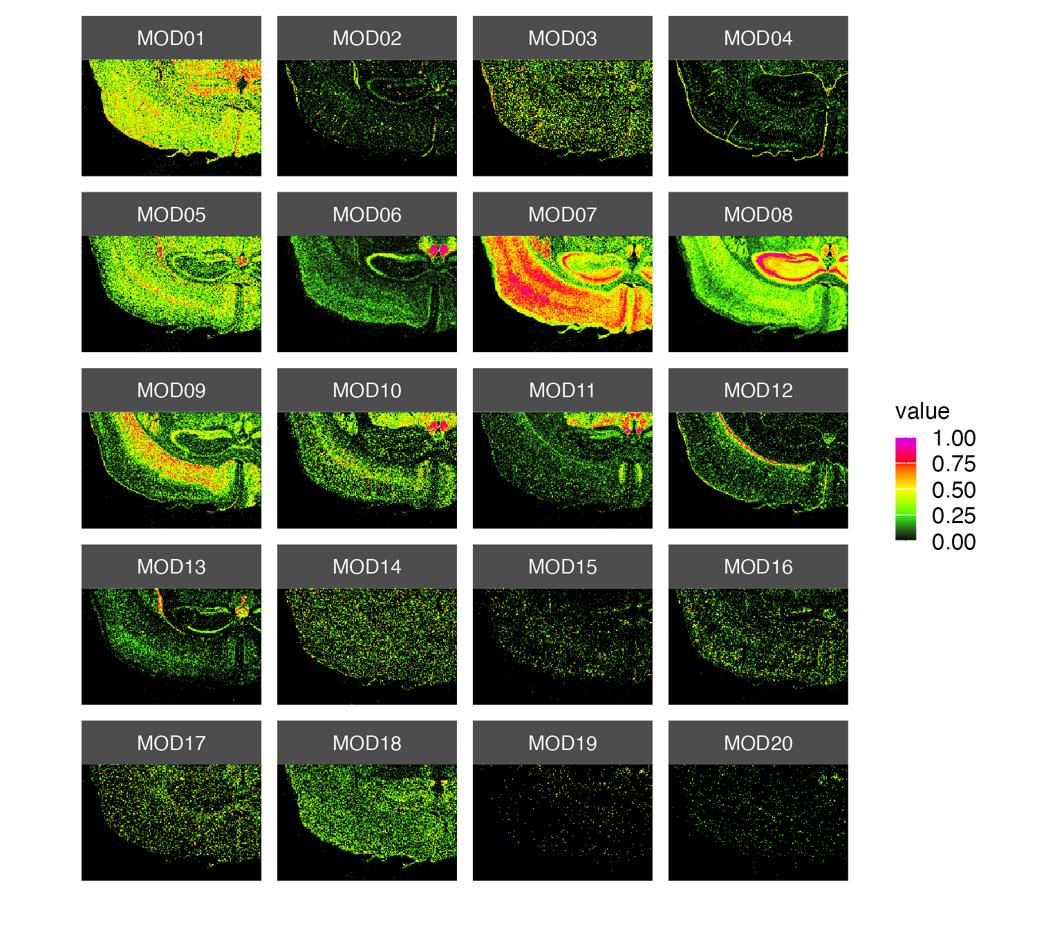

We can also plot the genes belonging to a specific module.

spatial_image(st_obj, features = hc_st$tree_classes[["MOD08"]], ncol = 3)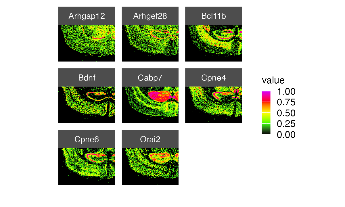

Assessing molecule clustering using Ripley’s K function

The STarlight package proposes the Ripley’s K function (from spatstat.explore package) to assess if gene molecules tend to be more concentrated or dispersed across the tissue. Users can use the compute_k_ripley function to get a list of genes whose molecules are spatially concentrated. For this tutorial, we chose to compute Ripley’s K function for a few genes because this step is rather time consuming as the molecule density increases.

plot_rip_k(compute_k_ripley(st_obj, rmax = 80, verbose = FALSE))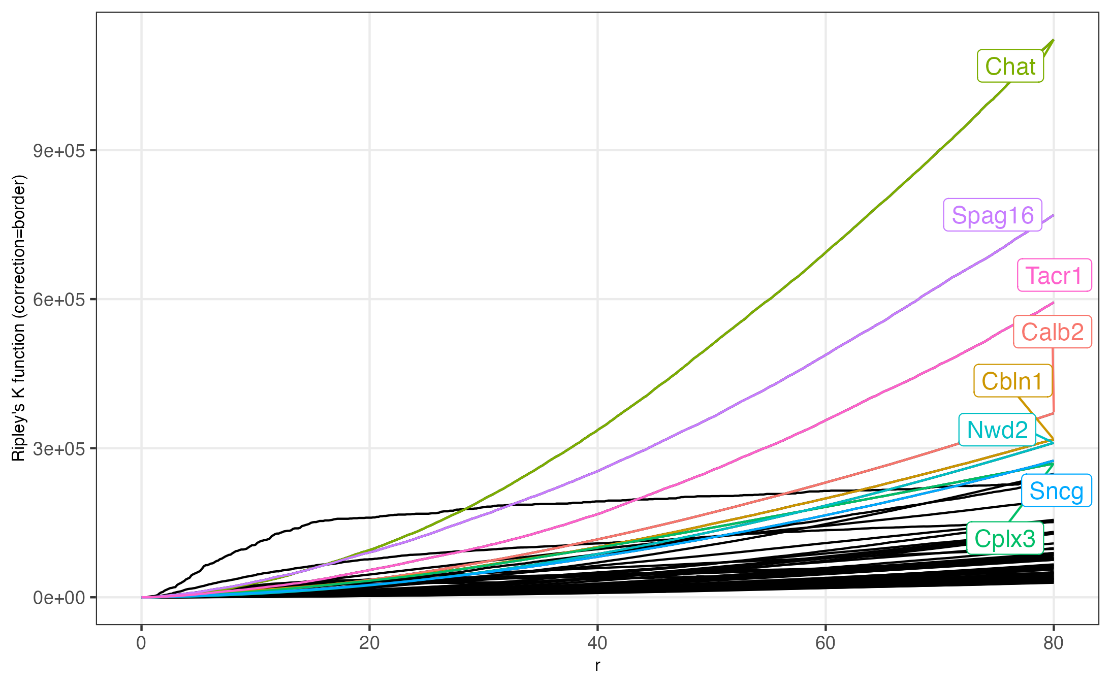

Mapping the above genes confirms they are spatially concentrated.


spatial_image(st_obj, features = c("Chat", "Spag16", "Tacr1", "Calb2"), ncol = 2)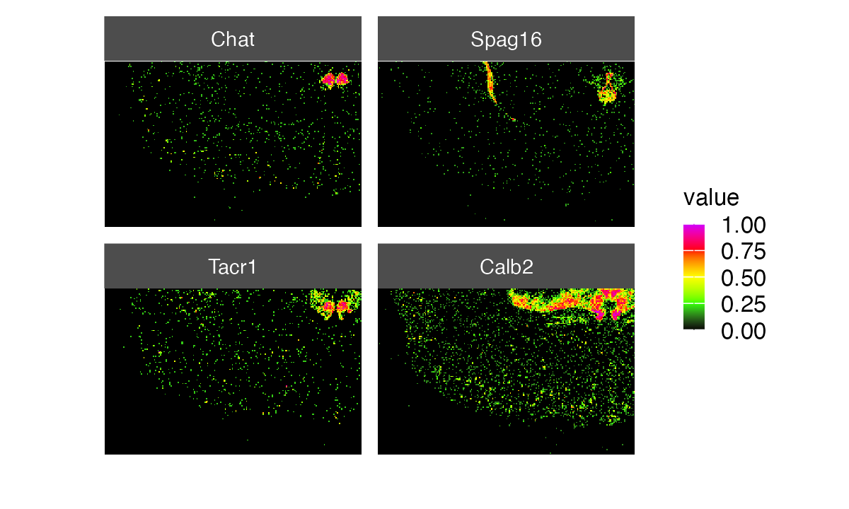

Dataset comparison: the STCompR class

Users can create an STCompR object from their STGrid object(s) using the stcompr() function. This object can then be used to easily compare multiple datasets. For illustrative purposes and to limit the computation time required for this vignette, we will compare two regions of the organ, which will be considered here as two conditions. We have chosen to generate two replicates per region (representative of two close regions).

Creating sample datasets

## "Region 1 = Condition 1"
# "replicate 1"
x_bins <-  bin_x(st_obj)[180:nbin_x(st_obj)]
y_bins <-  bin_y(st_obj)[100:nbin_y(st_obj)]
st_obj_r1_1 <- st_obj[x_bins, y_bins]

# "replicate 2"
x_bins <-  bin_x(st_obj)[170:200]
y_bins <-  bin_y(st_obj)[90:130]
st_obj_r1_2 <- st_obj[x_bins, y_bins]


## "Region 2 = Condition 2"
# "replicate 1"
x_bins <-  bin_x(st_obj)[60:100]
y_bins <-  bin_y(st_obj)[100:nbin_y(st_obj)]
st_obj_r2_1 <- st_obj[x_bins, y_bins]

# "replicate 2"
x_bins <-  bin_x(st_obj)[50:90]
y_bins <-  bin_y(st_obj)[80:130]
st_obj_r2_2 <- st_obj[x_bins, y_bins]

These are the datasets were are working with:

cmp_images(st_obj_r1_1,
           st_obj_r1_2,
           st_obj_r2_1, 
           st_obj_r2_2,
           feat_list="count_sum",
           names=c("region_1_1", "region_1_2", "region_2_1", "region_2_2"),
           color_y_strip=c("#3FA0FF", "#ABF8FF", "#EF6C00", "#FFB74D"),
           color_strip_text_y = "black",
           color_x_strip="#333333",
           colors = viridis::magma(10)
           )

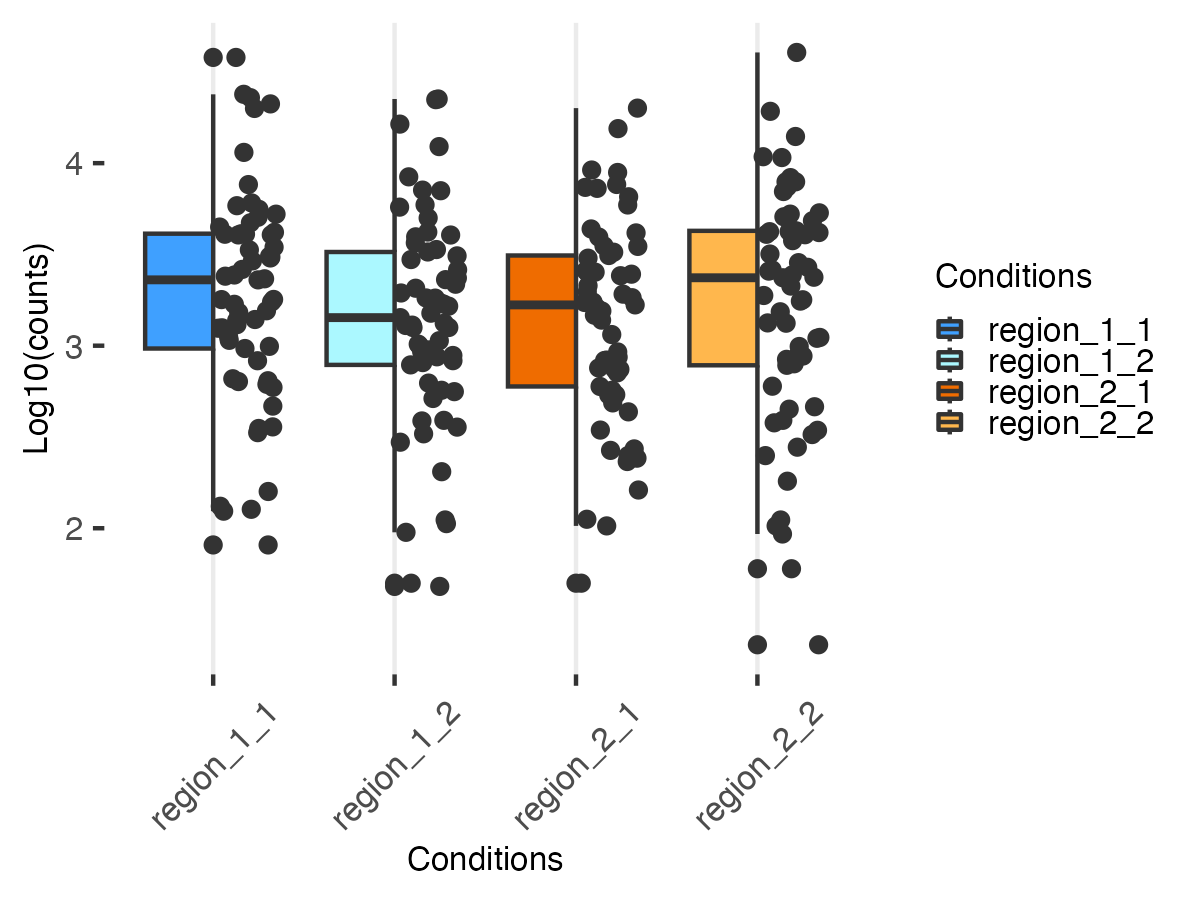
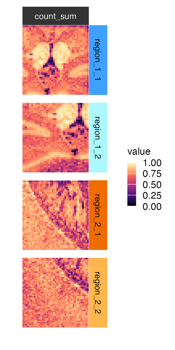We can visualize the count distribution for each replicate:

dist_st(
  st_obj_r1_1,
  st_obj_r1_2,
  st_obj_r2_1,
  st_obj_r2_2,
  transform = "log10",
  fill_color = c("#3FA0FF", "#ABF8FF", "#EF6C00", "#FFB74D"),
  names = c("region_1_1", "region_1_2", "region_2_1", "region_2_2")
)

Creating an STCompR object

Now we can create an STCompR object using the stcompr() function.

cmp <- stcompr(list(st_obj_r1_1,
                    st_obj_r1_2),
                list(st_obj_r2_1, 
                    st_obj_r2_2), 
               name_1="region_1", name_2="region_2")
#> gene-wise dispersion estimates
#> mean-dispersion relationship
#> final dispersion estimates

Count distribution

We can visualize the normalized count distribution for each replicate:

cmp_boxplot(cmp,
            transform = "log10",
            normalized = TRUE) + 
  scale_fill_manual(
              name = "Conditions",
              labels = c("region_1_1", "region_1_2", "region_2_1", "region_2_2"),
              values = c("#3FA0FF", "#ABF8FF", "#EF6C00", "#FFB74D")
            ) + 
  theme(axis.text.x = element_text(size = 8),
        axis.text.y = element_text(size = 8))
#> Scale for fill is already present.
#> Adding another scale for fill, which will replace the existing scale.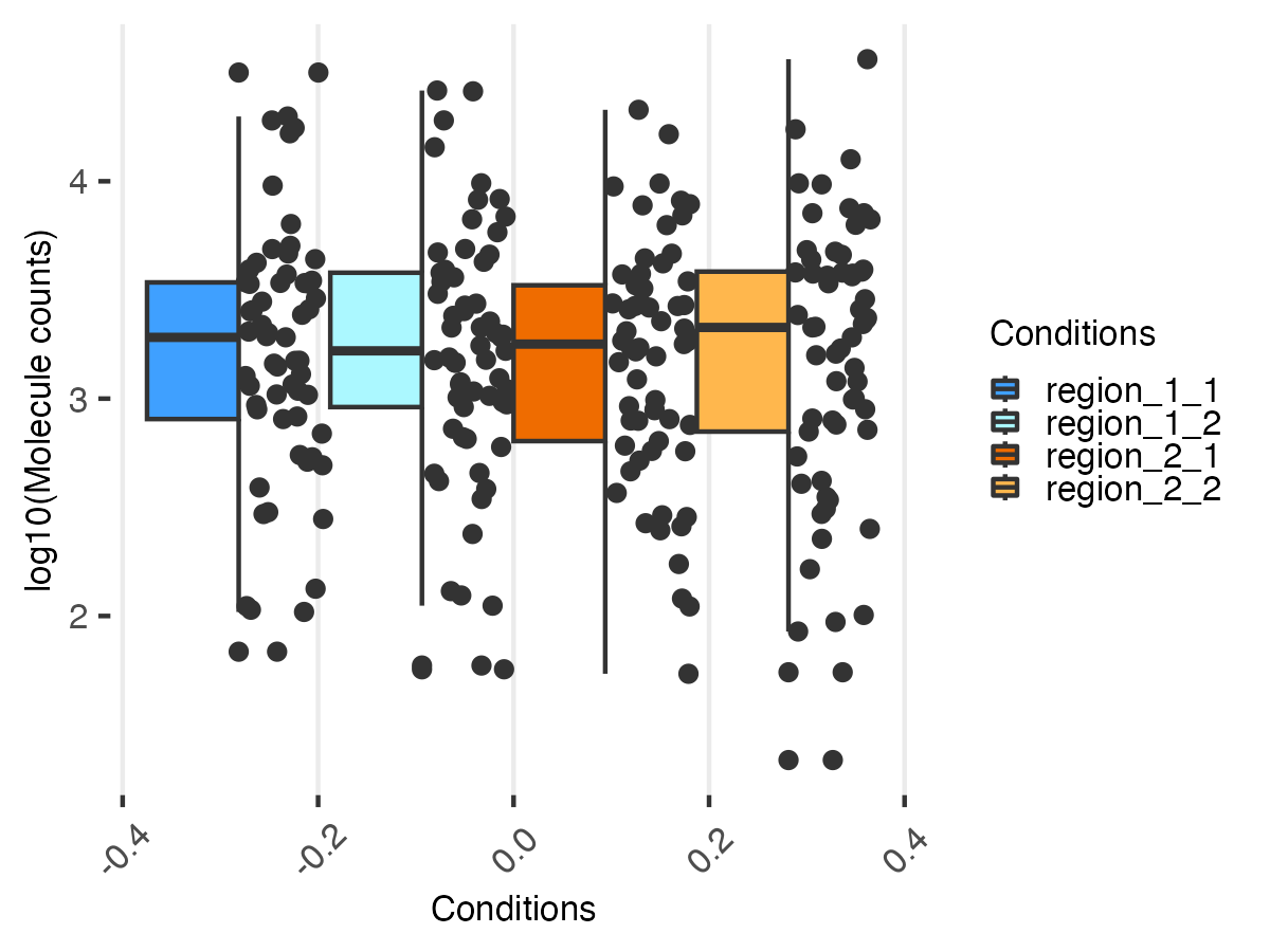

Count comparison

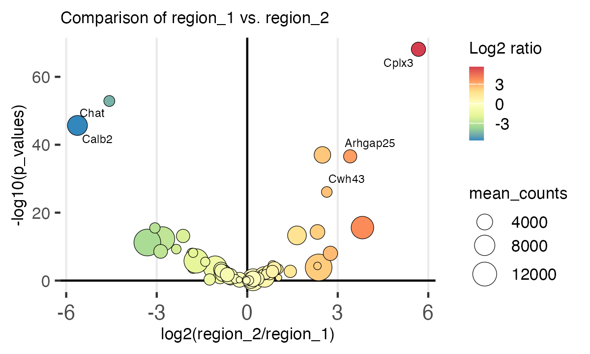
As we can see below, the expression level of several genes differ between both regions.

cmp_volcano(
  cmp,
  text_y_lim = 20,
  text_size = 2,
  text_x_lim = 2.5,
  title = "Comparison of region_1 vs. region_2"
)

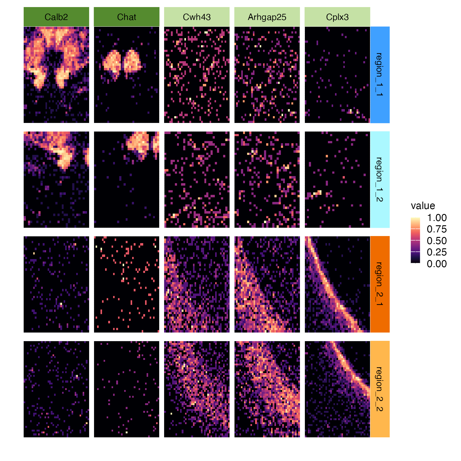
Using the cmp_images() function, we map these genes to see how they spatially differ across regions.

genes <- cmp@stat_test %>%
  dplyr::filter(abs(log2_ratio) > 2.5) %>%
  dplyr::arrange(log2_ratio) %>%
  dplyr::filter(-log10(p_values) > 20) %>% rownames()

cmp_images(
  st_obj_r1_1,
  st_obj_r1_2,
  st_obj_r2_1,
  st_obj_r2_2,
  feat_list = genes,
  names = c("region_1_1", "region_1_2", "region_2_1", "region_2_2"),
  color_y_strip = c("#3FA0FF", "#ABF8FF", "#EF6C00", "#FFB74D"),
  color_strip_text_y = "black",
  color_x_strip = c("#558B2F", "#558B2F", "#C5E1A5", "#C5E1A5", "#C5E1A5"),
  color_strip_text_x = "black",
  colors = viridis::magma(10)
)

Session info

sessioninfo::session_info()%>%
  details::details(
    summary = 'Current session info',
    open    = TRUE
  )

Current session info


 [1m [36m─ Session info ─────────────────────────────────────────────────────────────── [39m [22m
  [3m [90msetting  [39m [23m  [3m [90mvalue [39m [23m
 version  R version 4.3.3 (2024-02-29)
 os       macOS Sonoma 14.3.1
 system   x86_64, darwin20
 ui       X11
 language en
 collate  en_US.UTF-8
 ctype    en_US.UTF-8
 tz       Europe/Paris
 date     2024-09-18
 pandoc   3.1.11 @ /Applications/RStudio.app/Contents/Resources/app/quarto/bin/tools/x86_64/ (via rmarkdown)

 [1m [36m─ Packages ─────────────────────────────────────────────────────────────────── [39m [22m
  [3m [90mpackage              [39m [23m  [3m [90m* [39m [23m  [3m [90mversion    [39m [23m  [3m [90mdate (UTC) [39m [23m  [3m [90mlib [39m [23m  [3m [90msource [39m [23m
 abind                  1.4-5       [90m2016-07-21 [39m  [90m[2] [39m  [90mCRAN (R 4.3.0) [39m
 ape                    5.7-1       [90m2023-03-13 [39m  [90m[2] [39m  [90mCRAN (R 4.3.0) [39m
 aplot                  0.2.2       [90m2023-10-06 [39m  [90m[2] [39m  [90mCRAN (R 4.3.0) [39m
 Biobase                2.62.0      [90m2023-10-24 [39m  [90m[2] [39m  [90mBioconductor [39m
 BiocGenerics           0.48.1      [90m2023-11-01 [39m  [90m[2] [39m  [90mBioconductor [39m
 BiocParallel           1.36.0      [90m2023-10-24 [39m  [90m[2] [39m  [90mBioconductor [39m
 bit                    4.0.5       [90m2022-11-15 [39m  [90m[2] [39m  [90mCRAN (R 4.3.0) [39m
 bit64                  4.0.5       [90m2020-08-30 [39m  [90m[2] [39m  [90mCRAN (R 4.3.0) [39m
 bitops                 1.0-7       [90m2021-04-24 [39m  [90m[2] [39m  [90mCRAN (R 4.3.0) [39m
 bslib                  0.6.1       [90m2023-11-28 [39m  [90m[2] [39m  [90mCRAN (R 4.3.0) [39m
 cachem                 1.0.8       [90m2023-05-01 [39m  [90m[2] [39m  [90mCRAN (R 4.3.0) [39m
 cli                    3.6.2       [90m2023-12-11 [39m  [90m[2] [39m  [90mCRAN (R 4.3.0) [39m
 clipr                  0.8.0       [90m2022-02-22 [39m  [90m[2] [39m  [90mCRAN (R 4.3.0) [39m
 cluster                2.1.6       [90m2023-12-01 [39m  [90m[2] [39m  [90mCRAN (R 4.3.3) [39m
 codetools              0.2-19      [90m2023-02-01 [39m  [90m[2] [39m  [90mCRAN (R 4.3.3) [39m
 colorspace             2.1-0       [90m2023-01-23 [39m  [90m[2] [39m  [90mCRAN (R 4.3.0) [39m
 colourpicker           1.3.0       [90m2023-08-21 [39m  [90m[2] [39m  [90mCRAN (R 4.3.0) [39m
 cowplot                1.1.3       [90m2024-01-22 [39m  [90m[2] [39m  [90mCRAN (R 4.3.2) [39m
 crayon                 1.5.2       [90m2022-09-29 [39m  [90m[2] [39m  [90mCRAN (R 4.3.0) [39m
 data.table             1.15.2      [90m2024-02-29 [39m  [90m[2] [39m  [90mCRAN (R 4.3.2) [39m
 DBI                    1.2.2       [90m2024-02-16 [39m  [90m[2] [39m  [90mCRAN (R 4.3.2) [39m
 DelayedArray           0.28.0      [90m2023-10-24 [39m  [90m[2] [39m  [90mBioconductor [39m
 deldir                 2.0-4       [90m2024-02-28 [39m  [90m[2] [39m  [90mCRAN (R 4.3.2) [39m
 desc                   1.4.3       [90m2023-12-10 [39m  [90m[2] [39m  [90mCRAN (R 4.3.0) [39m
 DESeq2                 1.42.1      [90m2024-03-06 [39m  [90m[2] [39m  [90mBioconductor 3.18 (R 4.3.3) [39m
 details                0.3.0       [90m2022-03-27 [39m  [90m[2] [39m  [90mCRAN (R 4.3.0) [39m
 digest                 0.6.35      [90m2024-03-11 [39m  [90m[2] [39m  [90mCRAN (R 4.3.2) [39m
 dotCall64              1.1-1       [90m2023-11-28 [39m  [90m[2] [39m  [90mCRAN (R 4.3.0) [39m
 dplyr                * 1.1.4       [90m2023-11-17 [39m  [90m[2] [39m  [90mCRAN (R 4.3.0) [39m
 ellipsis               0.3.2       [90m2021-04-29 [39m  [90m[2] [39m  [90mCRAN (R 4.3.0) [39m
 envnames               0.4.1       [90m2020-12-08 [39m  [90m[2] [39m  [90mCRAN (R 4.3.0) [39m
 evaluate               0.23        [90m2023-11-01 [39m  [90m[2] [39m  [90mCRAN (R 4.3.0) [39m
 fansi                  1.0.6       [90m2023-12-08 [39m  [90m[2] [39m  [90mCRAN (R 4.3.0) [39m
 farver                 2.1.1       [90m2022-07-06 [39m  [90m[2] [39m  [90mCRAN (R 4.3.0) [39m
 fastDummies            1.7.3       [90m2023-07-06 [39m  [90m[2] [39m  [90mCRAN (R 4.3.0) [39m
 fastmap                1.1.1       [90m2023-02-24 [39m  [90m[2] [39m  [90mCRAN (R 4.3.0) [39m
 fitdistrplus           1.1-11      [90m2023-04-25 [39m  [90m[2] [39m  [90mCRAN (R 4.3.0) [39m
 fs                     1.6.3       [90m2023-07-20 [39m  [90m[2] [39m  [90mCRAN (R 4.3.0) [39m
 future                 1.33.1      [90m2023-12-22 [39m  [90m[2] [39m  [90mCRAN (R 4.3.0) [39m
 future.apply           1.11.1      [90m2023-12-21 [39m  [90m[2] [39m  [90mCRAN (R 4.3.0) [39m
 generics               0.1.3       [90m2022-07-05 [39m  [90m[2] [39m  [90mCRAN (R 4.3.0) [39m
 GenomeInfoDb           1.38.8      [90m2024-03-15 [39m  [90m[2] [39m  [90mBioconductor 3.18 (R 4.3.3) [39m
 GenomeInfoDbData       1.2.11      [90m2024-03-21 [39m  [90m[2] [39m  [90mBioconductor [39m
 GenomicRanges          1.54.1      [90m2023-10-29 [39m  [90m[2] [39m  [90mBioconductor [39m
 ggfun                  0.1.4       [90m2024-01-19 [39m  [90m[2] [39m  [90mCRAN (R 4.3.0) [39m
 ggh4x                  0.2.8       [90m2024-01-23 [39m  [90m[2] [39m  [90mCRAN (R 4.3.2) [39m
 ggnewscale             0.4.10      [90m2024-02-08 [39m  [90m[2] [39m  [90mCRAN (R 4.3.2) [39m
 ggplot2              * 3.5.0       [90m2024-02-23 [39m  [90m[2] [39m  [90mCRAN (R 4.3.2) [39m
 ggplotify              0.1.2       [90m2023-08-09 [39m  [90m[2] [39m  [90mCRAN (R 4.3.0) [39m
 ggpol                  0.0.7       [90m2020-11-08 [39m  [90m[2] [39m  [90mCRAN (R 4.3.0) [39m
 ggrepel                0.9.5       [90m2024-01-10 [39m  [90m[2] [39m  [90mCRAN (R 4.3.0) [39m
 ggridges               0.5.6       [90m2024-01-23 [39m  [90m[2] [39m  [90mCRAN (R 4.3.2) [39m
 ggsci                  3.0.1       [90m2024-03-02 [39m  [90m[2] [39m  [90mCRAN (R 4.3.2) [39m
 ggtree                 3.10.1      [90m2024-02-25 [39m  [90m[2] [39m  [90mBioconductor 3.18 (R 4.3.3) [39m
 globals                0.16.3      [90m2024-03-08 [39m  [90m[2] [39m  [90mCRAN (R 4.3.2) [39m
 glue                   1.7.0       [90m2024-01-09 [39m  [90m[2] [39m  [90mCRAN (R 4.3.0) [39m
 goftest                1.2-3       [90m2021-10-07 [39m  [90m[2] [39m  [90mCRAN (R 4.3.0) [39m
 gridExtra              2.3         [90m2017-09-09 [39m  [90m[2] [39m  [90mCRAN (R 4.3.0) [39m
 gridGraphics           0.5-1       [90m2020-12-13 [39m  [90m[2] [39m  [90mCRAN (R 4.3.0) [39m
 gtable                 0.3.4       [90m2023-08-21 [39m  [90m[2] [39m  [90mCRAN (R 4.3.0) [39m
 highr                  0.10        [90m2022-12-22 [39m  [90m[2] [39m  [90mCRAN (R 4.3.0) [39m
 htmltools              0.5.7       [90m2023-11-03 [39m  [90m[2] [39m  [90mCRAN (R 4.3.0) [39m
 htmlwidgets            1.6.4       [90m2023-12-06 [39m  [90m[2] [39m  [90mCRAN (R 4.3.0) [39m
 httpuv                 1.6.14      [90m2024-01-26 [39m  [90m[2] [39m  [90mCRAN (R 4.3.2) [39m
 httr                   1.4.7       [90m2023-08-15 [39m  [90m[2] [39m  [90mCRAN (R 4.3.0) [39m
 ica                    1.0-3       [90m2022-07-08 [39m  [90m[2] [39m  [90mCRAN (R 4.3.0) [39m
 igraph                 2.0.3       [90m2024-03-13 [39m  [90m[2] [39m  [90mCRAN (R 4.3.2) [39m
 IRanges                2.36.0      [90m2023-10-24 [39m  [90m[2] [39m  [90mBioconductor [39m
 irlba                  2.3.5.1     [90m2022-10-03 [39m  [90m[2] [39m  [90mCRAN (R 4.3.0) [39m
 jquerylib              0.1.4       [90m2021-04-26 [39m  [90m[2] [39m  [90mCRAN (R 4.3.0) [39m
 jsonlite               1.8.8       [90m2023-12-04 [39m  [90m[2] [39m  [90mCRAN (R 4.3.0) [39m
 KernSmooth             2.23-22     [90m2023-07-10 [39m  [90m[2] [39m  [90mCRAN (R 4.3.3) [39m
 knitr                  1.45        [90m2023-10-30 [39m  [90m[2] [39m  [90mCRAN (R 4.3.0) [39m
 labeling               0.4.3       [90m2023-08-29 [39m  [90m[2] [39m  [90mCRAN (R 4.3.0) [39m
 later                  1.3.2       [90m2023-12-06 [39m  [90m[2] [39m  [90mCRAN (R 4.3.0) [39m
 lattice                0.22-5      [90m2023-10-24 [39m  [90m[2] [39m  [90mCRAN (R 4.3.3) [39m
 lazyeval               0.2.2       [90m2019-03-15 [39m  [90m[2] [39m  [90mCRAN (R 4.3.0) [39m
 leiden                 0.4.3.1     [90m2023-11-17 [39m  [90m[2] [39m  [90mCRAN (R 4.3.0) [39m
 lifecycle              1.0.4       [90m2023-11-07 [39m  [90m[2] [39m  [90mCRAN (R 4.3.0) [39m
 listenv                0.9.1       [90m2024-01-29 [39m  [90m[2] [39m  [90mCRAN (R 4.3.2) [39m
 lmtest                 0.9-40      [90m2022-03-21 [39m  [90m[2] [39m  [90mCRAN (R 4.3.0) [39m
 locfit                 1.5-9.9     [90m2024-03-01 [39m  [90m[2] [39m  [90mCRAN (R 4.3.2) [39m
 magrittr             * 2.0.3       [90m2022-03-30 [39m  [90m[2] [39m  [90mCRAN (R 4.3.0) [39m
 MASS                   7.3-60.0.1  [90m2024-01-13 [39m  [90m[2] [39m  [90mCRAN (R 4.3.3) [39m
 Matrix                 1.6-5       [90m2024-01-11 [39m  [90m[2] [39m  [90mCRAN (R 4.3.3) [39m
 MatrixGenerics         1.14.0      [90m2023-10-24 [39m  [90m[2] [39m  [90mBioconductor [39m
 matrixStats            1.2.0       [90m2023-12-11 [39m  [90m[2] [39m  [90mCRAN (R 4.3.0) [39m
 memoise                2.0.1       [90m2021-11-26 [39m  [90m[2] [39m  [90mCRAN (R 4.3.0) [39m
 mgc                    2.0.2       [90m2020-06-23 [39m  [90m[2] [39m  [90mCRAN (R 4.3.0) [39m
 mime                   0.12        [90m2021-09-28 [39m  [90m[2] [39m  [90mCRAN (R 4.3.0) [39m
 miniUI                 0.1.1.1     [90m2018-05-18 [39m  [90m[2] [39m  [90mCRAN (R 4.3.0) [39m
 munsell                0.5.0       [90m2018-06-12 [39m  [90m[2] [39m  [90mCRAN (R 4.3.0) [39m
 nlme                   3.1-164     [90m2023-11-27 [39m  [90m[2] [39m  [90mCRAN (R 4.3.3) [39m
 parallelly             1.37.1      [90m2024-02-29 [39m  [90m[2] [39m  [90mCRAN (R 4.3.2) [39m
 patchwork            * 1.2.0       [90m2024-01-08 [39m  [90m[2] [39m  [90mCRAN (R 4.3.0) [39m
 pbapply                1.7-2       [90m2023-06-27 [39m  [90m[2] [39m  [90mCRAN (R 4.3.0) [39m
 pillar                 1.9.0       [90m2023-03-22 [39m  [90m[2] [39m  [90mCRAN (R 4.3.0) [39m
 pkgconfig              2.0.3       [90m2019-09-22 [39m  [90m[2] [39m  [90mCRAN (R 4.3.0) [39m
 pkgdown                2.0.9       [90m2024-04-18 [39m  [90m[2] [39m  [90mCRAN (R 4.3.2) [39m
 plotly                 4.10.4      [90m2024-01-13 [39m  [90m[2] [39m  [90mCRAN (R 4.3.0) [39m
 plyr                   1.8.9       [90m2023-10-02 [39m  [90m[2] [39m  [90mCRAN (R 4.3.0) [39m
 png                    0.1-8       [90m2022-11-29 [39m  [90m[2] [39m  [90mCRAN (R 4.3.0) [39m
 polyclip               1.10-6      [90m2023-09-27 [39m  [90m[2] [39m  [90mCRAN (R 4.3.0) [39m
 progressr              0.14.0      [90m2023-08-10 [39m  [90m[2] [39m  [90mCRAN (R 4.3.0) [39m
 promises               1.2.1       [90m2023-08-10 [39m  [90m[2] [39m  [90mCRAN (R 4.3.0) [39m
 purrr                  1.0.2       [90m2023-08-10 [39m  [90m[2] [39m  [90mCRAN (R 4.3.0) [39m
 R.methodsS3            1.8.2       [90m2022-06-13 [39m  [90m[2] [39m  [90mCRAN (R 4.3.0) [39m
 R.oo                   1.26.0      [90m2024-01-24 [39m  [90m[2] [39m  [90mCRAN (R 4.3.2) [39m
 R.utils                2.12.3      [90m2023-11-18 [39m  [90m[2] [39m  [90mCRAN (R 4.3.0) [39m
 R6                     2.5.1       [90m2021-08-19 [39m  [90m[2] [39m  [90mCRAN (R 4.3.0) [39m
 ragg                   1.3.0       [90m2024-03-13 [39m  [90m[2] [39m  [90mCRAN (R 4.3.2) [39m
 RANN                   2.6.1       [90m2019-01-08 [39m  [90m[2] [39m  [90mCRAN (R 4.3.0) [39m
 raster                 3.6-26      [90m2023-10-14 [39m  [90m[2] [39m  [90mCRAN (R 4.3.0) [39m
 RColorBrewer           1.1-3       [90m2022-04-03 [39m  [90m[2] [39m  [90mCRAN (R 4.3.0) [39m
 Rcpp                   1.0.12      [90m2024-01-09 [39m  [90m[2] [39m  [90mCRAN (R 4.3.0) [39m
 RcppAnnoy              0.0.22      [90m2024-01-23 [39m  [90m[2] [39m  [90mCRAN (R 4.3.2) [39m
 RcppHNSW               0.6.0       [90m2024-02-04 [39m  [90m[2] [39m  [90mCRAN (R 4.3.2) [39m
 RCurl                  1.98-1.14   [90m2024-01-09 [39m  [90m[2] [39m  [90mCRAN (R 4.3.0) [39m
 reshape2               1.4.4       [90m2020-04-09 [39m  [90m[2] [39m  [90mCRAN (R 4.3.0) [39m
 reticulate             1.35.0      [90m2024-01-31 [39m  [90m[2] [39m  [90mCRAN (R 4.3.2) [39m
 rlang                  1.1.3       [90m2024-01-10 [39m  [90m[2] [39m  [90mCRAN (R 4.3.0) [39m
 rmarkdown              2.26        [90m2024-03-05 [39m  [90m[2] [39m  [90mCRAN (R 4.3.2) [39m
 ROCR                   1.0-11      [90m2020-05-02 [39m  [90m[2] [39m  [90mCRAN (R 4.3.0) [39m
 RSpectra               0.16-1      [90m2022-04-24 [39m  [90m[2] [39m  [90mCRAN (R 4.3.0) [39m
 Rtsne                  0.17        [90m2023-12-07 [39m  [90m[2] [39m  [90mCRAN (R 4.3.0) [39m
 S4Arrays               1.2.1       [90m2024-03-06 [39m  [90m[2] [39m  [90mBioconductor 3.18 (R 4.3.3) [39m
 S4Vectors              0.40.2      [90m2023-11-23 [39m  [90m[2] [39m  [90mBioconductor [39m
 sass                   0.4.8       [90m2023-12-06 [39m  [90m[2] [39m  [90mCRAN (R 4.3.0) [39m
 scales                 1.3.0       [90m2023-11-28 [39m  [90m[2] [39m  [90mCRAN (R 4.3.0) [39m
 scattermore            1.2         [90m2023-06-12 [39m  [90m[2] [39m  [90mCRAN (R 4.3.0) [39m
 sctransform            0.4.1       [90m2023-10-19 [39m  [90m[2] [39m  [90mCRAN (R 4.3.0) [39m
 sessioninfo            1.2.2       [90m2021-12-06 [39m  [90m[2] [39m  [90mCRAN (R 4.3.0) [39m
 Seurat               * 5.1.0       [90m2024-05-10 [39m  [90m[2] [39m  [90mCRAN (R 4.3.3) [39m
 SeuratObject         * 5.0.2       [90m2024-05-08 [39m  [90m[2] [39m  [90mCRAN (R 4.3.2) [39m
 shiny                  1.8.0       [90m2023-11-17 [39m  [90m[2] [39m  [90mCRAN (R 4.3.0) [39m
 shinydashboard         0.7.2       [90m2021-09-30 [39m  [90m[2] [39m  [90mCRAN (R 4.3.0) [39m
 sp                   * 2.1-3       [90m2024-01-30 [39m  [90m[2] [39m  [90mCRAN (R 4.3.2) [39m
 spam                   2.10-0      [90m2023-10-23 [39m  [90m[2] [39m  [90mCRAN (R 4.3.0) [39m
 SparseArray            1.2.4       [90m2024-02-11 [39m  [90m[2] [39m  [90mBioconductor 3.18 (R 4.3.2) [39m
 spatstat.data          3.0-4       [90m2024-01-15 [39m  [90m[2] [39m  [90mCRAN (R 4.3.0) [39m
 spatstat.explore       3.2-6       [90m2024-02-01 [39m  [90m[2] [39m  [90mCRAN (R 4.3.2) [39m
 spatstat.geom          3.2-9       [90m2024-02-28 [39m  [90m[2] [39m  [90mCRAN (R 4.3.2) [39m
 spatstat.random        3.2-3       [90m2024-02-29 [39m  [90m[2] [39m  [90mCRAN (R 4.3.2) [39m
 spatstat.sparse        3.0-3       [90m2023-10-24 [39m  [90m[2] [39m  [90mCRAN (R 4.3.0) [39m
 spatstat.utils         3.0-4       [90m2023-10-24 [39m  [90m[2] [39m  [90mCRAN (R 4.3.0) [39m
 STarlight            * 0.0.9       [90m2024-09-18 [39m  [90m[1] [39m  [90mBioconductor [39m
 stringi                1.8.3       [90m2023-12-11 [39m  [90m[2] [39m  [90mCRAN (R 4.3.0) [39m
 stringr                1.5.1       [90m2023-11-14 [39m  [90m[2] [39m  [90mCRAN (R 4.3.0) [39m
 SummarizedExperiment   1.32.0      [90m2023-10-24 [39m  [90m[2] [39m  [90mBioconductor [39m
 survival               3.5-8       [90m2024-02-14 [39m  [90m[2] [39m  [90mCRAN (R 4.3.3) [39m
 systemfonts            1.0.6       [90m2024-03-07 [39m  [90m[2] [39m  [90mCRAN (R 4.3.2) [39m
 tensor                 1.5         [90m2012-05-05 [39m  [90m[2] [39m  [90mCRAN (R 4.3.0) [39m
 terra                  1.7-71      [90m2024-01-31 [39m  [90m[2] [39m  [90mCRAN (R 4.3.2) [39m
 textshaping            0.3.7       [90m2023-10-09 [39m  [90m[2] [39m  [90mCRAN (R 4.3.0) [39m
 tibble                 3.2.1       [90m2023-03-20 [39m  [90m[2] [39m  [90mCRAN (R 4.3.0) [39m
 tidyr                  1.3.1       [90m2024-01-24 [39m  [90m[2] [39m  [90mCRAN (R 4.3.2) [39m
 tidyselect             1.2.1       [90m2024-03-11 [39m  [90m[2] [39m  [90mCRAN (R 4.3.2) [39m
 tidytree               0.4.6       [90m2023-12-12 [39m  [90m[2] [39m  [90mCRAN (R 4.3.3) [39m
 treeio                 1.26.0      [90m2023-10-24 [39m  [90m[2] [39m  [90mBioconductor [39m
 utf8                   1.2.4       [90m2023-10-22 [39m  [90m[2] [39m  [90mCRAN (R 4.3.0) [39m
 uwot                   0.1.16      [90m2023-06-29 [39m  [90m[2] [39m  [90mCRAN (R 4.3.0) [39m
 vctrs                  0.6.5       [90m2023-12-01 [39m  [90m[2] [39m  [90mCRAN (R 4.3.0) [39m
 viridis                0.6.5       [90m2024-01-29 [39m  [90m[2] [39m  [90mCRAN (R 4.3.2) [39m
 viridisLite            0.4.2       [90m2023-05-02 [39m  [90m[2] [39m  [90mCRAN (R 4.3.0) [39m
 withr                  3.0.0       [90m2024-01-16 [39m  [90m[2] [39m  [90mCRAN (R 4.3.0) [39m
 xfun                   0.42        [90m2024-02-08 [39m  [90m[2] [39m  [90mCRAN (R 4.3.2) [39m
 xml2                   1.3.6       [90m2023-12-04 [39m  [90m[2] [39m  [90mCRAN (R 4.3.0) [39m
 xtable                 1.8-4       [90m2019-04-21 [39m  [90m[2] [39m  [90mCRAN (R 4.3.0) [39m
 XVector                0.42.0      [90m2023-10-24 [39m  [90m[2] [39m  [90mBioconductor [39m
 yaml                   2.3.8       [90m2023-12-11 [39m  [90m[2] [39m  [90mCRAN (R 4.3.0) [39m
 yulab.utils            0.1.4       [90m2024-01-28 [39m  [90m[2] [39m  [90mCRAN (R 4.3.2) [39m
 zlibbioc               1.48.2      [90m2024-03-13 [39m  [90m[2] [39m  [90mBioconductor 3.18 (R 4.3.3) [39m
 zoo                    1.8-12      [90m2023-04-13 [39m  [90m[2] [39m  [90mCRAN (R 4.3.0) [39m

 [90m [1] /private/var/folders/zy/wl3dj2_n76zfc8sdvny1q06c0000gn/T/Rtmpqvrydk/temp_libpath1001266f709b3 [39m
 [90m [2] /Library/Frameworks/R.framework/Versions/4.3-x86_64/Resources/library [39m

 [1m [36m────────────────────────────────────────────────────────────────────────────── [39m [22m

Denis Puthier & Jessica Chevallier

2024-02-07