Color-coded representation of the object (e.g. molecules) density — spatial

This function displays a color-coded representation of the object (e.g. molecules) density observed in a spatial transcriptomics experiment.

# S4 method for STGrid
spatial_image(
  object = NULL,
  features = NULL,
  saturation = 1,
  scale = TRUE,
  colors = c("black", "#33FF00", "#FFFF00", "#FF0000", "#CC00FF"),
  coord_fixed = TRUE,
  overlay_feature = NULL,
  colors_overlay = c("#DEEBF7", "#9ECAE1", "#3182BD", "blue"),
  grid_by = NULL,
  color_grid = "white",
  size = 0.5,
  logb = 10,
  pseudo_count = 1,
  as_factor = FALSE,
  ncol = 4
)

Arguments

object: The STGrid object.
features: The name of the features for which the spatial image will be created.
saturation: The ceiling level for the feature expression values. Defaults to 1 (no ceiling).
scale: Logical value indicating whether to scale the feature expression values. Defaults to TRUE.
colors: The colors to use for gradient fill in the spatial image. Defaults to a set of colors.
coord_fixed: Logical value indicating whether to keep the aspect ratio fixed. Defaults to TRUE.
overlay_feature: The feature to overlay on the spatial image. Defaults to NULL.
colors_overlay: The colors to use for gradient fill in the overlay feature. Defaults to a set of colors.
grid_by: Whether to overlay a grid with horizontal and vertical lines at particular interval. No overlay if NULL otherwise the size of the interval (e.g. 20).
color_grid: A color for the grid.
size: The size of the overlayed points.
logb: The basis for the log transformation. Default to 10. If NULL no log transformation.
pseudo_count: a value for the pseudo count used for log transformation (default to 1).
as_factor: Whether to consider the feature as a factor (e.g. for ggplot scale).
ncol: The number of columns for the facets.

Examples

example_dataset()
xen <- Xenium_Mouse_Brain_Coronal_7g
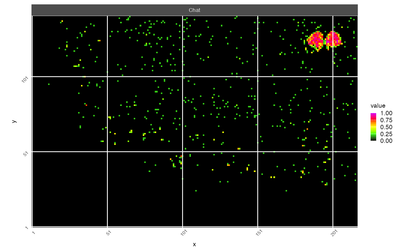
spatial_image(xen,
             features="Chat",
             grid_by=50)

bx <- bin_x(xen)[175:nbin_x(xen)]
by <- bin_y(xen)[100:nbin_y(xen)]
sub <- xen[bx, by]
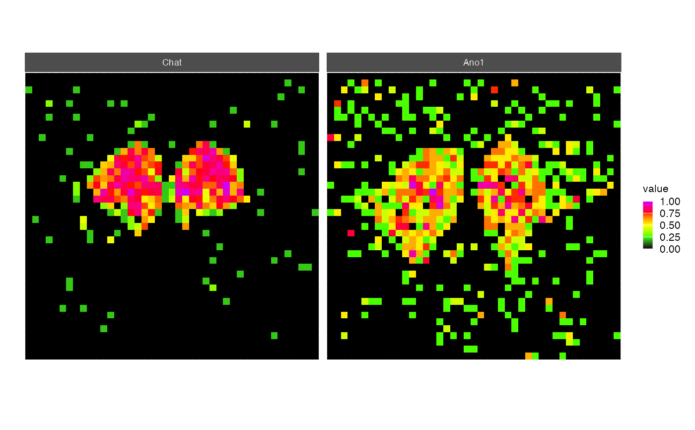
spatial_image(sub,
             features=c("Chat", "Ano1"))

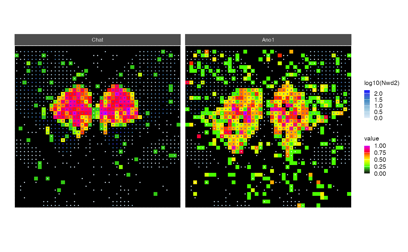
spatial_image(sub,
             features=c("Chat", "Ano1"),
             overlay_feature="Nwd2",
             size=0.05)