Create a barplot to show counts for selected features.

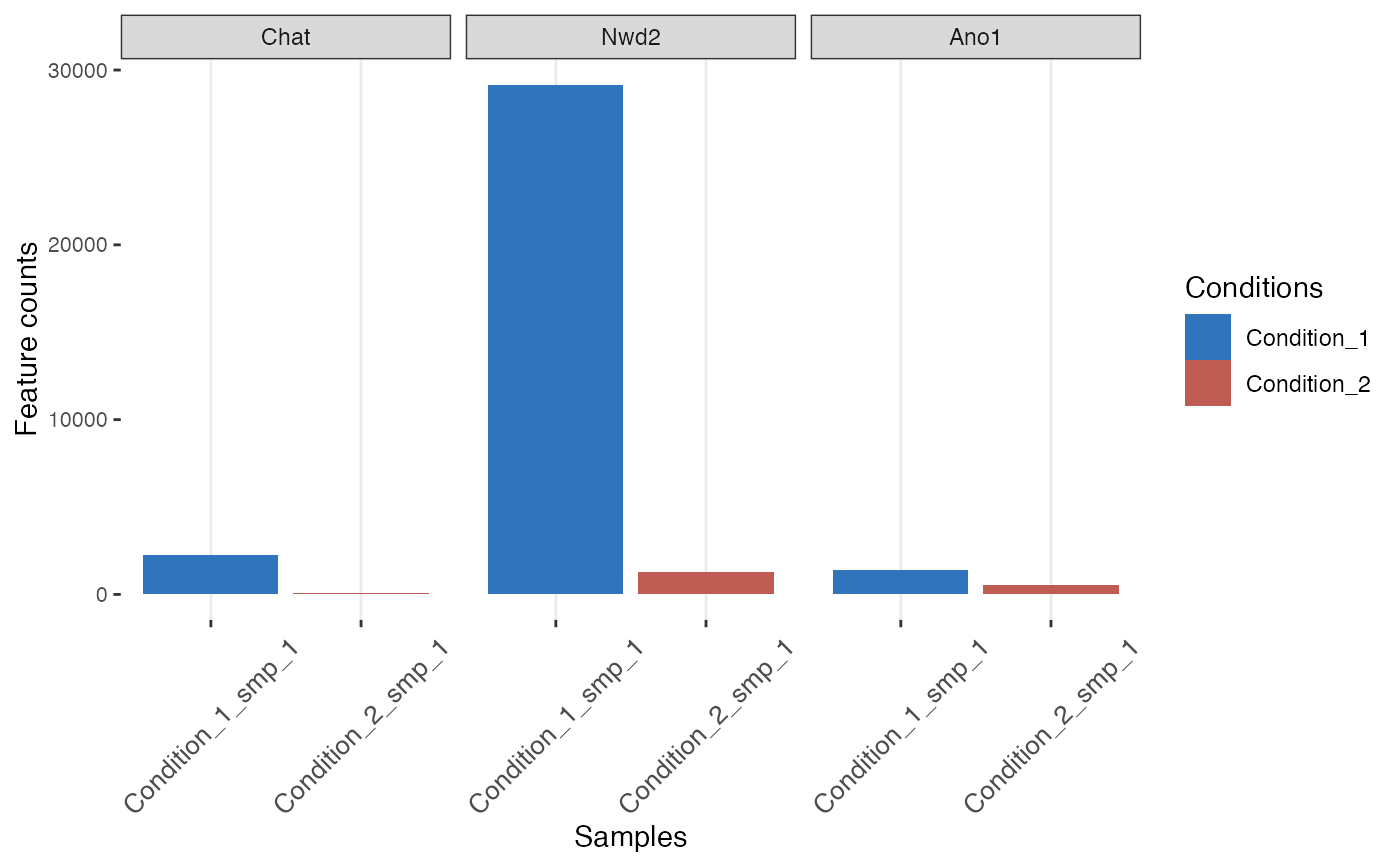
Create a barplot to show counts for selected features.

cmp_bar_plot(
  object,
  features = utils::head(feat_names(object)),
  normalized = FALSE,
  transform = c("None", "log2", "log10", "log"),
  colors = c("#3074BB", "#BE5B52")
)

Arguments

object

A STGrid object.

features

The list of features (NULL for all of them).

normalized

Whether counts should be normalized.

transform

Whether the count should be transformed (the pseudo count defined for the object is added).

colors

A set of colors.

Examples

example_dataset()
#> |-- INFO :  Dataset 11284233/files/Xenium_Mouse_Brain_Coronal_7g was already loaded. 
xen <- Xenium_Mouse_Brain_Coronal_7g
x_bins <-  bin_x(xen)[181:nbin_x(xen)]
y_bins <-  bin_y(xen)[101:nbin_y(xen)]
xen_r1 <- xen[x_bins, y_bins]
x_bins <-  bin_x(xen)[61:101]
y_bins <-  bin_y(xen)[101:nbin_y(xen)]
xen_r2 <- xen[x_bins, y_bins]
cmp <- stcompr(xen_r1, xen_r2)
#> |-- INFO :  Checking objects. 
#> |-- INFO :  Objects were provided as STGrid 
#> |-- INFO :  Converting to lists. 
#> |-- INFO :  Checking feature names. 
#> |-- INFO :  Retrieving counts. 
#> |-- INFO :  Merging counts. 
#> |-- INFO :  Normalizing counts... 
#> |-- INFO :  Only two samples. Performing Fisher's exact test. 
#> |-- INFO :  Preparing an STCompR object...  
cmp_bar_plot(cmp,
             features=c("Chat", "Nwd2", "Ano1"))