Statistics for Bioinformatics - Practicals - Gene enrichment statistics
Denis Puthier & Jacques van Helden
2 Nov 2015
Introduction
In this practical, we will inspect the statistical tests used to compare a set of genes of interest to a set of reference genes. This practical is essentially a tutorial, based on the result returned by David in the previous practical Handling genomic coordinates.
In this tutorial, we hade submitted a set of predicted E2F target genesc(see file M00920_targets.txt) to the Web tool DAVID, to compare it to various catalogues of functional annotations (Gene Ontology, KEGG, …). DAVID returned a table reporting the functional classes for which our gene set showed significant enrichment.
The goal of this tutorial is to reproduce the calculation of the significance. We will show two distinct ways to model the problem:
- Hypergeometric test: drawing at random a certain number of balls from an urn containing marked and non-marked balls (hypergeometric test).
- Fisher’s exact test: testing the independence between regulation (genes belonging or not to the E2F predicted gene set) and class membership (genes annotated or not as involved in cell cycle, in the GO annotations).
Click to open the image in a separate window 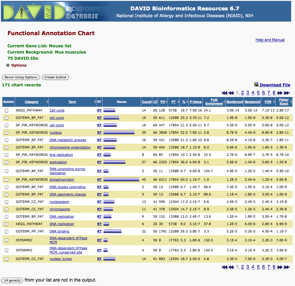
Tutorial
Hypergeometric test
In a first time, we model the association between genes and GO class using a hypergeometric distribution. The classical example for the hypergeometric is the ranomd selection of “k” balls in an urn containing “m” marked and “n” non-marked balls, and the observation that the selection contains “x” marked ball.
To illustrate the way to perform the hypergeometric test, we will re-analyze the second row of the David result displayed above: correspondence between a set of predicted E2F target genes and the genes annotated in the functional class “cell cycle” of the GOTERM_BP_FAT terms.
We define the parameters of the hypergeometric test in the following way:
Variable Description \(m = 611\) number of “marked” elements, i.e. total number of genes annotated for the selected GO term (cell cycle in GOTERM_BP_FAT annotations). \(N = 13588\) total number of genes with some annotation in GOTERM_BP_FAT. Note: this is lower than the total number of human genes, since many genes are of totally unknown function. \(n = N - m\) number of “non-marked” elements, i.e. the number of genes that have some annotation in GOERM_BP_FAT, but are not associated to the selected GO term (cell cycle). \(k = 59\) Size of the selection, i.e. number of genes predicted as E2F targets, and associated to at least one “Biological Process” in the Gene Ontology. \(x = 19\) number of “marked” elements in the selection, i.e. number of genes predicted as E2F targets AND associated to the process “cell cycle” in GO annotations.
g <- 75 ## Number of submitted genes
k <- 59 ## Size of the selection, i.e. submitted genes with at least one annotation in GO biological processes
m <- 611 ## Number of "marked" elements, i.e. genes associated to this biological process
N <- 13588 ## Total number of genes with some annotation in GOTERM_BP_FAT.
n <- N - m ## Number of "non-marked" elements, i.e. genes not associated to this biological process
x <- 19 ## Number of "marked" elements in the selection, i.e. genes of the group of interest that are associated to this biological process
Small exercise: random expectation
Compute the following statistics:
- the percent of the gene selection involved in the process.
- the percentage of the biological process covered by our gene selection.
- expected number of marked elements in the selection
- “fold enrichment”.
Answer
## Percent of the gene selection involved in "cell cycle". This
## corresponds to the "%" column returned by DAVID.
(percent.selection <- x / g * 100)
## [1] 25.33333## Percent, among submitted genes with at least one annotation, which
## are involved in "cell cycle".
(percent.selection <- x / k * 100) ## [1] 32.20339## Percent of the biological process covered by the gene set.
(percent.process <- x / m * 100) ## [1] 3.109656## Random expectation
(marked.proportion <- m / N)## [1] 0.04496615(exp.x <- k * marked.proportion)## [1] 2.653003## Fold enrichment, as computed by David
(fold.enrichment <- (x / k ) / (m / N)) ## [1] 7.161697Interpretation
The calculation of the proportion of marked genes indicates that 4.5% of the genes annotated in GO_BP_FAT are associated to cell cycle. It is not surprizing that cell cycle is mobilizing an important fraction of the gene products, this was already shown for yeast in a pioneering microarray study (Spellmann et al., 1998).
Our selection contains 59 genes with at least some annotation in GO_BP_FAT. If we would have selected 59 genes at random, we would thus expect 59*4.5% of them to be annotated as “cell cycle”.
Drawing the hypergeometric distribution
Use the plot() and the dhyper() functions to draw the distribution of probability densities, i.e. the probability to observe a particular value of \(x\): \(P(X=x)\).
## Define the range of possible values for x.
## The number of marked elements in the selection can neither be
## higher than the size of the selection, nor higher than the
## number of marked elements.
x.range <- 0:min(k,m)

help(dhyper) ## Always read the documentation of a function before using it.

## Compute the distribution of density P(X=x)
dens <- dhyper(x=x.range, m=m, n=n, k=k)

## Plot the distributon of hypergeometric densities
plot (x.range, dens, type="h", lwd=2, col="blue", main="Hypergeometric density", xlab="x = marked elements in the selection", ylab="density = P(X=x)", ylim=c(0, max(dens)*1.25))

## Draw an arrow indicating the expected value
arrows(exp.x, max(dens)*1.15, exp.x, max(dens)*1.05, lwd=2, col='darkgreen', angle=30, length=0.1, code=2)
text(exp.x, max(dens)*1.20, labels=paste("exp=", round(exp.x, digits=2)), col="darkgreen", font=2)

## Draw an arrow indicating the observed value
arrows(x, max(dens)*1.15, x, max(dens)*1.05, lwd=2, col='red', angle=30, length=0.1, code=2)
text(x, max(dens)*1.20, labels=paste("x=", x), col="red", font=2)
Interpretation
With the parameters of our analysis, the hypergeometric density function has an asymmetric bell shape (in other cases, the distribution can be j-shaped or i-hsaped, or have a symmetrical bell shape). The red arrows indicates the number of E2F target genes which are annotated as “cell cycle”. The hystogram already shows us an obvious fact: this number is much higher than what would be expected by chance (exp = 2.65), and it seems to have a very low probability.
A better way to emphasize small values is to plot the ordinates (Y axis) on a logarithmic scale.
## Plot the probability distribution with logarithmic axes
plot (x.range, dhyper(x=x.range, m=m, n=n, k=k), type="l", lwd=2, col="blue", main="Hypergeometric density (log Y scale)", xlab="x = marked elements in the selection", ylab="density = P(X=x)", log="y", panel.first=grid())

## Arrow indicating expected value
arrows(exp.x, max(dens)*1e-10, exp.x, max(dens)*1e-2, lwd=2, col='darkgreen', angle=30, length=0.1, code=2)
text(exp.x, max(dens)*1e-15, labels=paste("exp=", round(exp.x, digits=2)), col="darkgreen", font=2)

## Arrow indicating observed value
arrows(x, dens[x+1]*1e-10, x, dens[x+1]*1e-2, lwd=2, col='red', angle=30, length=0.1, code=2)
text(x, dens[x+1]*1e-15, labels=paste("x=", x), col="red", font=2)
This logarithmic plot shows that the probability decreases very rapidly when the number of marked elements exceeds the expectation. In particular, the probability to observe by chance a selection made of marked elements only is very low (2e-81):
print(dhyper(x=k, m=m, n=n, k=k))## [1] 2.080018e-81Computing the hypergeometric P-value
The P-value is the probability to observe at least “x” marked balls in the selection.
Compute the P-value for the observed number of marked elements in the selection
p.value <- phyper(q=x -1, m=m, n=n, k=k, lower.tail=FALSE)Explanation
- By default, the R function phyper computes the inclusive lower tail of the distribution: P(X ≤ x).
- With the option “lower.tail=FALSE”, phyper() returns the exclusive upper tail P(X>x).
- We want the *inclusive* upper tail : P-value = P(X≥x). For this, we can compute the exclusive upper tail of the value just below x. Indeed, since the distribution is discrete, P(X >x-1) = P(X ≥x).
We suggest you to read the documentation to check that the reasoning above is correct.
help(phyper)## Compute the distribution of P-values (for all possible values of x).
p.values <- phyper(q=x.range -1, m=m, n=n, k=k, lower.tail=FALSE)
## Plot the P-value distribution on linear scales
plot(x.range, p.values, type="l", lwd=2, col="violet", main="Hypergeometric P-value", xlab="x = marked elements in the selection", ylab="P-value = P(X>=x)", ylim=c(0, 1), panel.first=grid())
## Arrow indicating observed value
arrows(x, max(dens)*1.35, x, max(dens)*1.1, lwd=2, col='red', angle=30, length=0.1, code=2)
text(x, max(dens)*1.5, labels=paste("x=", x, "; p-val=", signif(digits=1, p.value), sep=""), col="red", font=2)
## We can plot the density below the P-value
lines(x.range, dens, type="h", col="blue", lwd=2)
legend("topright", legend=c("P-value", "density"), lwd=2, col=c("violet", "blue"), bg="white", bty="o")
To better emphasize small P-values, we will display the P-value distribution with a logarithmic ordinate.
## Plot the P-value distribution with a logarithmic Y scale

plot(x.range, p.values,  type="l", lwd=2, col="violet", main="Hypergeometric P-value (log Y scale)", xlab="x = marked elements in the selection", ylab="P-value = P(X>=x); log scale", panel.first=grid(), log='y')

## Arrow indicating observed value
arrows(x, p.value, x, min(dens), lwd=2, col='red', angle=30, length=0.1, code=2)
text(x, min(dens), labels=paste("x=", x, sep=""), col="red", font=2, pos=4)

## Arrow indicating the P-value
arrows(x, p.value, 0, p.value, lwd=2, col='red', angle=30, length=0.1, code=2)
text(0, p.value*1e-5, labels=paste("p-val=", signif(digits=2, p.value), sep=""), col="red", font=2, pos=4)
Questions
Did we obtain the same P-value as DAVID ? If not, read David help page and try to understand the reason for the difference.
This will be further discussed during the practicals.
Fisher’s exact test
## Prepare a two-dimensional contingency table
contingency.table <- data.frame(matrix(nrow=2, ncol=2))
rownames(contingency.table) <- c("predicted.target", "non.predicted")
colnames(contingency.table) <- c("class.member", "non.member")

## Assign the values one by one to make sure we put them in the right
## place (this is not necessary, we could enter the 4 values in a
## single instruction).
contingency.table["predicted.target", "class.member"] <- x ## Number of marked genes in the selection
contingency.table["predicted.target", "non.member"] <- k - x ## Number of non-marked genes in the selection
contingency.table["non.predicted", "class.member"] <- m - x ## Number of marked genes outside of the selection
contingency.table["non.predicted", "non.member"] <- n - (k - x) ## Number of non-marked genes outside the selection


print(contingency.table)
## class.member non.member
## predicted.target 19 40
## non.predicted 592 12937## Print marginal sums
(contingency.row.sum <- apply(contingency.table, 1, sum))## predicted.target non.predicted
## 59 13529(contingency.col.sum <- apply(contingency.table, 2, sum))## class.member non.member
## 611 12977## Create a contingency table with marginal sums
contingency.table.margins <- cbind(contingency.table, contingency.row.sum)
contingency.table.margins <- rbind(contingency.table.margins, apply(contingency.table.margins, 2, sum))
names(contingency.table.margins) <- c(names(contingency.table), "total")
rownames(contingency.table.margins) <- c(rownames(contingency.table), "total")
print(contingency.table.margins)## class.member non.member total
## predicted.target 19 40 59
## non.predicted 592 12937 13529
## total 611 12977 13588## Check the total
print(sum(contingency.table)) ## The value shoudl equal N, since every## [1] 13588 ## possible gene must be assigned to one
## cell of the contingency table.
print(N)## [1] 13588## Run Fisher's exact test
ftest.result <- fisher.test(x=contingency.table, alternative="greater")
print(ftest.result)##
## Fisher's Exact Test for Count Data
##
## data: contingency.table
## p-value = 4.99e-12
## alternative hypothesis: true odds ratio is greater than 1
## 95 percent confidence interval:
## 6.204117 Inf
## sample estimates:
## odds ratio
## 10.37524attributes(ftest.result) ## Display the list of attribute of the object returned by ftest## $names
## [1] "p.value" "conf.int" "estimate" "null.value" "alternative"
## [6] "method" "data.name"
##
## $class
## [1] "htest"print (ftest.result$p.value) ## Print the P-value of the exact test## [1] 4.989683e-12################################################################
## Compute expected values in the contingency table
exp.contingency.table <- contingency.table ## Quick and dirty way to obtain the same structure as the original contingency table
exp.contingency.table[ ] <- contingency.row.sum %*% t(contingency.col.sum) / N
## Add row and column sums (marginal sums)
exp.contingency.table <- cbind(exp.contingency.table, contingency.row.sum)
exp.contingency.table <- rbind(exp.contingency.table, apply(exp.contingency.table, 2, sum))
names(exp.contingency.table) <- c(names(contingency.table), "total")
rownames(exp.contingency.table) <- c(rownames(contingency.table), "total")
print(exp.contingency.table)## class.member non.member total
## predicted.target 2.653003 56.347 59
## non.predicted 608.346997 12920.653 13529
## total 611.000000 12977.000 13588Interpretation
We applied a Fisher test to test the independence between two characteristics of the genes: the fact to belong or not to our gene selection (i.e. E2F predicted targets); the fact to be or not involved in cell cycle. The contincengy table indicates the actual distribution of the genes among those classes.
                 class.member non.member total
predicted.target           19         40    59
non.predicted             592      12937 13529
total                     611      12977 13588
Under the hypothesis of independence, we would expect to find the genes distributed randomly within the table, but with the same marginal sums. To achieve this, we can estimate the expected number of elements in each cell by taking the product of the total entries in the row and column, and dividing it by the total number of genes.
                 class.member non.member total
predicted.target     2.653003     56.347    59
non.predicted      608.346997  12920.653 13529
total              611.000000  12977.000 13588
The Fisher test measure the distance between the observed and the expected contingency table. The P-value indicates the probability to obtain by chance a distance at least as great as we do. When this P-value is very small, it means that it is very unlikely that the elements were distributed at random, and we reject the null hypothesis (hypothesis of independence).
In our case, this p-value is 7.08e-8, it is thus very unlikely that our two criteria (“E2F target genes” and “cell cycle”, resp) are independent. In other terms, small P-values indicate a significant association between the E2F target genes and the biological process “cell cycle”.
Note that the P-value returned by the Fisher test is identical to the P-value returned by the hypergeometric test above. Actually the Fisher test relies on the hypergeometrical distribution to compute its P-value. This P-value is also identical to the “Fisher” column in the result table of the Web tool DAVID.
Denis Puthier (TAGC, Aix-Marseille Université).
Jacques van Helden (TAGC, Aix-Marseille Université).